


 Download PDF
ABSTRACT
The investigations of anomalous transport involved the use of validated fluorescent-bead trajectories obtained within the H-actin networks with mesh sizes of 225 nm, 250 nm, 300 nm, 550 nm, 625 nm and 750 nm. After a structural quality control, the mean-squared displacement (MSD) curves of the individual trajectories were built using coordinate increments but keeping the units of original coordinates and the unit of the coordinate lag. For each of the six mesh-size conditions, objective fitting windows were selected to give the following empirical values for the scaling exponents, γ: 0.453412,0.460879,0.516736,0.856105,0.866278 and 0.920213 (γ), respectively, where sublinear transport occurred in all of the 6 cases. The robustness of these estimates was tested for 300 trajectory-level bootstrap resamples in each condition. The ensemble estimates were in good agreement with the bootstrap median exponents and empirical 95% intervals for these, reflecting the reproducibility of the main scaling behaviour. A strong empirical association was also observed between mesh size and γ, with an estimated slope of 0.000991 𝑛𝑚⁻¹ (𝑅² = 0.959861, 𝑝 = 0.000612, 𝑁 = 6).
Complementary, a fractional diffusion-reaction model was developed that includes the temporal order α, spatial order β, transport coefficient κ and relaxation/removal coefficient λ as well as a sensitivity-based local structural-identifiability framework. The mathematical form is used to highlight the parameter distinguishability, but there is not enough calibrated data in the released trajectory or a well-motivated observation operator, needed to recover all four mechanistic parameters numerically from the MSD alone. Hence, the empirical scaling found by the test and the proposed framework on fractional inverse-identification are presented separately.
Keywords: Anomalous Diffusion; Mean-Squared Displacement; H-Actin Networks; Fluorescent Bead Trajectories; Fractional Diffusion-Reaction Equation; Structural Identifiability; Parameter Sensitivity; Bootstrap Uncertainty; Inverse Problems; Single-Particle Tracking
ABSTRACT
The investigations of anomalous transport involved the use of validated fluorescent-bead trajectories obtained within the H-actin networks with mesh sizes of 225 nm, 250 nm, 300 nm, 550 nm, 625 nm and 750 nm. After a structural quality control, the mean-squared displacement (MSD) curves of the individual trajectories were built using coordinate increments but keeping the units of original coordinates and the unit of the coordinate lag. For each of the six mesh-size conditions, objective fitting windows were selected to give the following empirical values for the scaling exponents, γ: 0.453412,0.460879,0.516736,0.856105,0.866278 and 0.920213 (γ), respectively, where sublinear transport occurred in all of the 6 cases. The robustness of these estimates was tested for 300 trajectory-level bootstrap resamples in each condition. The ensemble estimates were in good agreement with the bootstrap median exponents and empirical 95% intervals for these, reflecting the reproducibility of the main scaling behaviour. A strong empirical association was also observed between mesh size and γ, with an estimated slope of 0.000991 𝑛𝑚⁻¹ (𝑅² = 0.959861, 𝑝 = 0.000612, 𝑁 = 6).
Complementary, a fractional diffusion-reaction model was developed that includes the temporal order α, spatial order β, transport coefficient κ and relaxation/removal coefficient λ as well as a sensitivity-based local structural-identifiability framework. The mathematical form is used to highlight the parameter distinguishability, but there is not enough calibrated data in the released trajectory or a well-motivated observation operator, needed to recover all four mechanistic parameters numerically from the MSD alone. Hence, the empirical scaling found by the test and the proposed framework on fractional inverse-identification are presented separately.
Keywords: Anomalous Diffusion; Mean-Squared Displacement; H-Actin Networks; Fluorescent Bead Trajectories; Fractional Diffusion-Reaction Equation; Structural Identifiability; Parameter Sensitivity; Bootstrap Uncertainty; Inverse Problems; Single-Particle Tracking
INTRODUCTION
Background and Scientific Motivation
There are physical and biological systems in which the displacement statistics do not follow the classical diffusive behavior of a Brownian motion, which is characterized by anomalous transport. Sub diffusive behavior is particularly seen as a sub linear mean-squared displacement (MSD) with lag time. The nonlocal temporal memory and, if necessary, spatial no locality are mathematical representations of such behavior that are provided by fractional differential equations [1-2].
A considerable amount of research has been done in both mathematical and physical formulations of fractional diffusion theory. The classical first order time derivative is replaced by a time-fractional operator, while a fractional spatial operator is used to represent different scales of spatial transport [1,3-5]. These properties have led to the use of fractional models as representations of transport processes that classical integer-order diffusion is not good enough to represent.
Another avenue for physical relevance of anomalous transport is found in actin based materials. To set the context for the transport regime that we consider here, experimental studies have reported anomalous sub diffusive behavior and anomalous local viscoelastic responses in actin networks [6].
Inverse-Problem Motivation
Forward simulation of a fractional diffusion model is unable to solve the inverse problem of estimating the unknown parameters in the model from observations. Recovering fractional orders and diffusion coefficients in fractional diffusion equations can be strongly dependent on the observation configuration and have significant ill conditioning [7,8]. Uniqueness and reconstruction results for selected combinations of fractional orders and physical parameters have been established under specific boundary, integral, or pointwise observation configurations [9–12].
The results presented here indicate that fractional parameters are identifiable under appropriate informative observations but also reveal that the identifiability of the parameters is related to the mathematical structure of the forward model and the available data. Thus, a good numerical match is not necessarily seen as being evidence for structural uniqueness.
Structural Identifiability
The issue of structural identifiability is when different sets of parameters can produce the same ideal observations. It is quite distinct from noisy or finite data practical parameter estimation, which is used more often. General structural-identifiability analysis has revealed that the model parameterization, measurement configuration and data nature can have a significant impact on parameter distinguishability [13-16].
In the case of fractional-order systems, several studies have focused on parameter identifiability by means of input-output information, coefficient mappings and sensitivity-based methods [17-18]. In recent years, the concept of structural-identifiability has been extended to networks with fractional order dynamics [19]. The results of these studies show that in practice, fractional-order models can have identifiable parameter combinations and can have strong practical conditioning or parameter confounding.
The present study therefore focuses on three related but also distinct questions: is a parameterization locally structurally identifiable, is the resulting sensitivity matrix well conditioned and can the parameters be stably estimated from available observations.
Experimental Anomalous-Diffusion Observations
The experimental source is not the trajectory of the actin material itself, but rather the trajectory of the fluorescent beads that are trapped in the networks (H- or F-actin). Trajectory matrices are released which include x-pixel location, y-pixel location and trajectory number. The impact of uncertainty in localization, finite trajectory length, temporal sampling, heterogeneity and statistical treatment on the transport properties inferred from the single particle tracking methodology is emphasized in modern approaches. Modern approaches are focusing on the impact of uncertainty in localization, finite length of trajectories, temporal sampling, heterogeneity and statistical treatment on the inferred transport properties [20]-[21].
This is why the present study considers the MSD exponent that is found experimentally as an empirical scaling parameter instead of assuming it to be equal to the fractional temporal order of the governing PDE. There is also a warning that different anomalous-diffusion mechanisms may yield the same power law in the MSD [22].
Research Gap
The literature provides a rich background for fractional differential equations [1,2,5,7-12] and their inverse problems [7-11] for identification of structure. It also contains structural-identifiability analysis methods for the fractional-order systems and networks [17-19] and theory that differentiates between structural and practical identifiability [13-16].
However, the literature reviewed here does not provide a directly validated observation map that converts the present bead-trajectory-derived MSD curves into a uniquely calibrated four-parameter space-time fractional diffusion-reaction inverse problem. The present study therefore extends the theoretical framework, but adheres to the strict separation of the process of empirical scaling and the process of parameter recovery.
Problem Statement
The model used in this research is the theoretical model called
Where In this case α is the temporal fractional order, β the spatial fractional order, κ the transport coefficient, λ an effective reaction or removal coefficient, A a positive spatial operator and g prescribed forcing. The model is constructed as a mathematical model, but the four model parameters are not estimated from the existing MSD data since the necessary calibrated observation operator is not given in the MSD data release.
Research Objectives
structure and trajectory level quality control of provided fluorescent-bead trajectory data;
Create objective window MSD scaling estimates and uncertainty at the trajectory level; and
Develop a forward model of fractional diffusion-reaction; and
Calculate parameter sensitivities and a local criterion for structural-identifiability of the theoretical parameter-to-observation map;
Determine the information needed to link the information from the trajectory-derived MSD to a fractional propagator; and
Do not attempt to numerically estimate α, β, κ and λ (when the experimental observation operator is not fully calibrated).
Contributions of The Present Study
The main contribution is a traceable integration of validated bead-trajectory analysis , uncertainty-aware MSD scaling, and a very explicit fractional diffusion-reaction identifiability framework. In addition the work shows a kind of methodological fence : with the present data, empirical anomalous scaling is supported, but a four-parameter mechanistic identification needs further calibrated observations or extra model assumptions, and these simply are not in the released trajectory archive.
Organization of The Manuscript
Section 2 presents the systematic literature review and the comparative evidence tables. Section 3 explains the experimental data, quality control, how the MSD is built, bootstrap analysis, the fractional model, the numerical framework, and the limits of the observation model. Section 4 develops the mathematical analysis and the local identifiability theory. Section 5 gives the graphical representation and a physical interpretation of the validated experimental results. Section 6 reports the experimental results and also discusses the implications and limitations of the fractional inverse framework. Section 7 summarizes the findings and the conclusions. The Appendix includes the full numerical datasets, audit tables, numerical validation protocols, and also the Google Colab code that was used during the analysis.
Literature Review
Systematic Literature-Review Protocol
A structured systematic literature review approach was used, to map literature relevant to fractional differential equations, anomalous diffusion, inverse fractional problems, parameter identification, structural identifiability, numerical approximation, and trajectory-based transport analysis. The evidence base was organized around peer-reviewed papers that in fact supported the theoretical or numerical aspect and the inverse-problem, identifiability and experimental angle of this study [1-39]. The review highlights newer results of the period 2021-2026, but retains older references where they are relevant, to nail down the established framework and theory, so to speak.
Fractional Diffusion and Anomalous Transport
Fractional Diffusion and Anomalous Transport Fractional differential equations provide a framework for representing nonlocal temporal memory and, where appropriate, spatial nonlocality in anomalous transport [1,2]. Spectral and finite-difference methods have been developed for time-fractional diffusion equations [3,4]. Regularity theory and L1-scheme analyses address numerical challenges associated with fractional memory [23,24]. On bounded domains, the definition of a fractional spatial operator depends on the chosen operator and boundary conditions; different definitions of the fractional Laplacian are not interchangeable [5].
The Structural and Practical Identifiability
The concept of structural identifiability is essentially the concept of uniqueness for the ideal cases of observation, while the concept of practical identifiability is related to the difficult cases of finite observation data, noisy as well [13-16]. A knowledge-based approach, based on input-output knowledge and structural-identifiability methods, has been used to inspect fractional-order systems [17-18]. Then, a new development was the extension of the same line of thinking to fractional order networks [19]. Taken together these works show why it is important to tease apart rank-based local identifiability, from numerical conditioning, in a clear way.
Trajectory Analysis And MSD
Recent reviews emphasize that localization uncertainty, finite trajectory lengths, temporal resolution, heterogeneity, and statistical treatment can affect transport estimates obtained from single-particle tracking [20,21]. The background for this subdiffusive (anomalous) behavior of the actin network has been provided by the experimental literature [6].
Inverse Fractional Diffusion
Studies on inverse fractional-diffusion, have looked into source recovery[7], also one-dimensional time fractional diffusion [8]. There is likewise fractional-order recovery [9], and even simultaneous potential / order recovery [10]. There are works that focus on fractional-order and time-dependent coefficient identification [11] and some that focus on the simultaneous uniqueness for fractional-order and diffusion related coefficients [12]. More generally, other papers tackle inverse coefficient issues that use Hilfer operators, plus coefficient/ source recovery, as well as singular-source configurations [25-28].
Numerical Inverse Methods
More recently, optimization, learning and numerical workflows for fractional parameter identifications have been addressed [29-31,39]. Spectral methods and finite-element discretizations, finite-difference schemes, L1 schemes, robust finite-difference schemes and ADI methods have been considered for the numerical approximation of the time-fractional diffusion [32-37]. Other Mittag-Leffler kernel formulations provide additional numerical perspectives [38] but are not used as the kernel in the model used here.
Comparative Evidence Table
The comparative evidence map is summarized in Table 1.
| Research area | Representative references | Established contribution | Limitation relative to present study |
|---|---|---|---|
| Fractional theory | [1-5,23-[24] | Operators, diffusion, numerical analysis | General theory; not our experimental inverse problem |
| Fractional identifiability | [17-19] | Fractional parameter distinguishability | Mostly finite-dimensional/network formulations |
| General identifiability | [13-16] | Structural vs practical identifiability | Not specific to current bead-MSD observation |
| Trajectory/MSD methods | [20-21] | SPT and MSD interpretation | Does not provide fractional PDE parameter identification |
| Actin transport | [6,22] | Experimental anomalous transport context | Does not establish our mechanistic inverse map |
| Inverse fractional PDEs | [7-12,25-28] | Source/order/coefficient recovery | Different unknown sets and observation configurations |
| Numerical identification | [29-31,39] | Optimization and learning approaches | Numerical recovery does not itself establish structural identifiability |
| Fractional PDE numerics | [32-38] | Forward discretization and convergence | Primarily numerical approximation |
Table 1: Systematic evidence map of literature relevant to the present study.
Research-Gap Matrix
Table 2 summarizes the research gaps and corresponding responses.
| Gap | Literature basis | Unresolved issue | Present response |
|---|---|---|---|
| Joint temporal and spatial fractional orders | [9-12] | Few studies connect both orders to bead-derived MSD | Present framework treats α and β explicitly but does not overclaim numerical identification |
| PDE-level structural identifiability | [13-19] | Existing literature is broader or finite-dimensional | Sensitivity-rank framework is developed conditionally for the PDE map |
| Trajectory-derived observation map | [20,21,22] | MSD is not a direct PDE state measurement | Observation bridge is identified as a required modeling component |
| Uncertainty-aware scaling | [20,21] | Trajectory dependence affects inference | 300 trajectory-level bootstrap replicates are used |
| Numerical verification | [23,24,32-37] | Fractional discretization requires convergence checks | Forward and sensitivity verification protocols are specified |
Table 2: Research-gap identification matrix
Contributions Relative to Prior Work
The principal contributions of the present study are summarized in Table 3.
| Contribution | Status | Description |
|---|---|---|
| Validated experimental MSD analysis | Current work | Six mesh-size conditions; objective windows; bootstrap uncertainty |
| Fractional forward framework | Current work | Caputo temporal order, spectral spatial operator, reaction/removal term |
| Sensitivity/identifiability theory | Current work | Local rank criterion, singular values, conditioning concepts |
| Observation-model audit | Current work | Explicit recognition that bead MSD is not automatically a PDE-state observation |
| Reproducible computational record | Current work | Frozen data manifests, complete observation tables, and Colab code in Appendix |
Table 3: Principal contributions of the present study.
Literature-Review Conclusion
The literature supports the mathematical and numerical foundations of the study, while also making clear that the experimental MSD cannot be converted automatically, into a fully calibrated four-parameter fractional PDE inverse problem. So, this contribution is positioned as a validated anomalous transport analysis coupled to a rigorous fractional identifiability framework, with the unresolved observation model bridge explicitly identified, rather than kept hidden or just implied, in the background.
Methodology
Overall Framework
Figure 1 summarizes the experimental-to-model workflow.
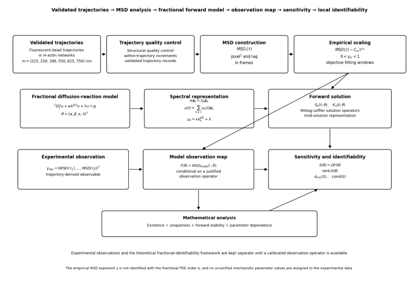
Figure 1: Integrated experimental-to-fractional inverse-identification workflow
Note: The workflow links validated fluorescent-bead trajectories in H-actin networks at (m={225,250,300,550,625,750},nm) to the empirical observation MSD m(t) and scaling exponent (γm), while the theoretical pathway introduces (θ=(α,β,κ,λ)T), the fractional state u(·,·;θ), and the sensitivity map (S(θ)=DF(θ)), thereby separating experimentally measured transport behavior from the theoretical identifiability framework without assigning unverified numerical values to (α,β,κ,λ).
Experimental Trajectory Data
The main set comprises fluorescent bead trajectories that were captured in H-actin/F-actin networks for six different mesh-size conditions: 225, 250, 300, 550, 625 and 750 nm. The released MAT matrices consist of an x pixel location, a y pixel location and also a trajectory number. The two additional structurally audited files are retained for provenance but are excluded from the primary six-condition MSD analysis. .
Trajectory quality control
There is a structural quality check that screens for rows, exact duplicate rows, trajectory-ID integrity, and also the statistics of trajectory length. For the six primary mesh-size datasets everything cleared the structural audit, with zero 𝑁𝑎𝑁/𝐼𝑛𝑓 rows and zero exact duplicate rows. A more detailed file-level manifest is provided in Appendix A, so anyone can verify it line by line if needed.
Mean-squared displacement
Consider a single trajectory r, with recorded position . The displacement over a lag τ can be expressed
The ensemble MSD is then
Important note, only increments that stay within the same trajectory are used not cross-trajectory differences, or other mixes like that. Also, the released coordinates remain in pixel units, and the lag stays in frame units because a confirmed physical space-and-time calibration is not included in the released trajectory matrices.
Only increments in the trajectory are counted. The released coordinate are kept in pixel units and the released lag is kept in frame units because there is no verified physical spatial and temporal calibration in the released trajectory matrices.
Objective scaling analysis
The empirical scaling model is over a chosen lag time interval.
Equivalently, . The selected windows are
7 − 69, 7 − 72, 3 − 100, 1 − 50, 1 − 46, and 1 − 23 frames for 225, 250, 300, 550, 625, and 750 nm, respectively. The selection of each window was done by the objective process described in the workbook.
Trajectory-level bootstrap
The uncertainty is evaluated by a re-sample with replacement and a repetition of the MSD and scaling analysis. For each mesh size condition, the frozen analysis is based on 300 trajectory level bootstrap replicates. The bootstrap summary and empirical intervals are given in Appendix B.
Fractional diffusion-reaction framework
The theoretical model is
Where
The model is set up as a theoretical framework for forward analysis and structural identifiability and it is not numerically identified from the current bead-MSD data.
Caputo derivative
The numerical solution of this memory term is based on the well known time-fractional discretization literature [23], [24].
Spectral fractional spatial operator
If A is an operator on a Hilbert space and {φk} is an orthonormal eigenbasis for A then let .
The spectral fractional power is:
Since the analysis of a fractional spatial operator on bounded domains is dependent on the choice of the operator and boundary conditions, the spectral construction is used.
Forward solution representation
With , the modal equation is . The solution operators are represented by Mittag-Leffler functions, and the solution is represented by a sum of these.
The parameter-to-state and observation spaces are introduced. The concept of parameter-to-state and observation spaces is introduced.
Parameter-to-state and observation spaces
The parameter-to-state map is the map . But what is actually observed in the experiment is the bead-trajectory MSD and not the PDE state itself. Thus, the map between the model and the data space should be conditionally defined as where
MSD_model is a propagator or observation functional which is justified.
Numerical discretization and verification of the accuracy of the results
A convolution approximation of type L1 is used for the benchmark forward verification, where the spectral representation of the spatial operator is used. The complete version of Google Colab is provided in Appendix D. The benchmark is carefully designed to be isolated from the experimental inversion and contains only known test parameters to verify the code.
Sensitivity Computation
Let zq be the partial derivative of u with respect to q, when it exists, for q = α, β, κ, λ The coefficient sensitivities are the differencing of the governing equation. The contents of the spectral factor are included in the β derivative.
Sensitivity Matrix
The Inverse Problem and The Identifiability Status
The data audit presented in this work does not give any information about the model-specific observation operator needed to compute J for the four mechanistic parameters, which is a general constrained inverse problem written as Therefore, there is no reported value of the unknown numerical value of θ̂. The identifiability criterion still hasn't been demonstrated in practice with real data, and is just a theoretical result of the model framework.
Mathematical Analysis
Functional setting
Let Ω be a bounded domain and X=L²(Ω). Let A be positive and self-adjoint with compact resolvent and eigenpairs 𝐴𝜑𝑘 = 𝜌𝑘𝜑𝑘. The spectral fractional operator is defined consistently with the bounded-domain spectral construction [5].
Fractional Evolution Problem
Modal Reduction
Mild Solution
Under the functional assumptions stated in Section 4.1, with 0 < 𝛼< 1, 𝜅> 0, 𝜆≥0, 𝑢0 ∈𝑋, and 𝑔∈𝐿2(0, 𝑇; 𝑋), the spectral fractional evolution problem admits a unique mild solution on [0,T]. The modal representation in (11) and the Mittag-Leffler solution in (12) provide the constructive representation of that solution. Consequently, existence and
uniqueness are established for the theoretical forward problem under the stated operator and regularity assumptions; these results do not imply experimental identifiability of the parameters from the present scalar MSD observations.
Existence and Uniqueness
Forward Stability
Parameter Continuity
Coefficient Sensitivities
Spatial-Order Sensitivity
Temporal-Order Sensitivity
The α direction requires stronger regularity because the parameter changes the fractional operator itself. In the computational verification,𝛼 sensitivity is treated numerically through centered finite differences; no complete operator-level differentiability theorem is claimed for the experimental setting.
Model-To-Observation Map
where L represents a mathematically justified observation functional. For the current bead-MSD data, the existence of a unique calibrated L is not established by the released dataset; this is therefore an explicit modeling limitation rather than a hidden assumption.
Sensitivity Matrix
The parameter-to-observation structure and sensitivity diagnostics are shown in Figure 2.
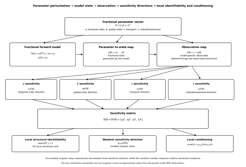
Figure 2: Mathematical Sensitivity-Identifiability Architecture
Note: The fractional parameter vector (θ = (α,β,κ,λ)T) generates the model state (u(·,·;θ)), which is mapped to the observable (F(θ)); the sensitivity matrix (S(θ) = DF(θ) = [∂αF, ∂βF, ∂κF, ∂λF]) represents the four parameter directions, while and rank S(θ*) = 4, σmin(S) > 0, cond2(S) = σmax(S)/σmin(S). characterize local distinguishability and conditioning without assigning unverified numerical values to (\alpha,\beta,\kappa,\lambda).
Local Structural Identifiability
A parameter θ* is locally structurally identifiable if F is locally one-t o-one near θ*. A sufficient condition under continuous differentiability is full column rank of the Jacobian.
Identifiability Theorem
If F is continuously differentiable near θ* and rank 𝐷𝐹(𝜃∗) = 4, then a four-component submap has a nonsingular Jacobian and the inverse function theorem yields local injectivity. This establishes local structural identifiability for the theoretical observation map, not automatic experimental identifiability from the present MSD dataset.
Sensitivity Gramian and Singular Values
The smallest singular value characterizes the weakest local sensitivity direction. The condition number is
Sensitivity Correlation
High correlation indicates potential parameter confounding, particularly for β and κ because both influence the spectral transport contribution. These metrics are theoretical diagnostics and are not populated with fabricated experimental values.
Mathematical Limitation
The current experiment provides MSD curves for the scalar, not spatially resolved, observations of the PDE state or a calibrated propagator. Therefore, the full rank condition is presented as a structural-identifiability condition in theory, and the four-parameter experimental recovery is still not included in the evidence supported by the present set of data.
Representing and Interpreting Results Graphically
Experimental MSD Curves
The bead trajectories are validated, and we get the MSD curve for 6 different mesh size conditions. Due to the lack of spatial calibration in the released coordinate archive the MSD is still in pixel² and lag is still in frame units. Direct empirical basis for the analysis of anomalous transport is given by the curves.
Log-Log Scaling Representation
The empirical relation between 𝑀𝑆𝐷𝑚(𝜏)and 𝜏 is plotted on a log-log graph, with 𝐶𝑚 and 𝛾𝑚 as the constants. The value of the exponent 𝛾𝑚 is not automatically identified as the fractional order α, and is an empirical scaling descriptor.
The experimental MSD curves for the six mesh-size conditions are shown in Figure 3.
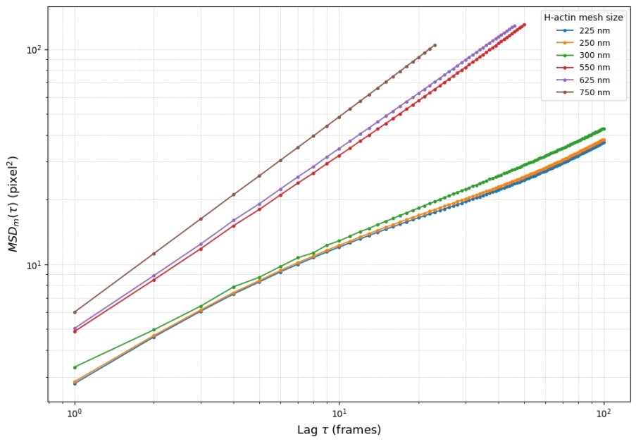
Figure 3: Experimental mean-squared displacement across H-actin mesh-size conditions.
Note: The validated fluorescent-bead trajectories at (m={225,250,300,550,625,750},nm) produce MSDm(τ) in pixel² versus lag (τ) in frames, with sublinear scaling characterized by (γm={0.453412,0.460879,0.516736,0.856105,0.866278,0.920213}); the increase of (γm) toward 1 indicates progressively less sublinear transport as mesh size increases, while no numerical values of the theoretical parameters (α,β,κ,λ) are assigned.
Objective-Window Scaling Results
The six ensemble exponents are γ = {0.453412,0.460879,0.516736,0.856105,0.866278,0.920213}The corresponding selected windows are 7-69, 7-72, 3-100, 1-50, 1-46, and 1-23 frames. These values are direct outputs of the frozen empirical analysis.
Bootstrap Uncertainty
The bootstrap medians are {0.453919,0.460630,0.517128,0.855996,0.866041,0.920303}, with empirical 95% intervals [0.446181,0.460032], [0.452920,0.468995], [0.508430,0.525142], [0.851258,0.861506], [0.855814,0.874961], and [0.914970,0.925160].
Window Sensitivity
Window sensitivity is strongest for the smaller mesh-size conditions and comparatively narrower at larger mesh sizes. The full duplicated window-sensitivity table is provided in Appendix C. The empirical association between mesh size and the MSD scaling exponent is illustrated in Figure 4.
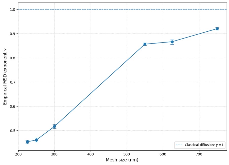
Figure 4: Mesh-size dependence of the empirical anomalous-diffusion exponent.
Figure 4: Mesh-size dependence of the empirical anomalous-diffusion exponent. For six conditions {225, 250, 300, 550, 625, 750} the ensemble exponent increases monotonically from 0.453412 to 0.920213. A linear trend gives a slope. Physically, the effective transport scaling becomes closer to the classical diffusive limit γ=1 as mesh size increases.
Physical Interpretation Of Γ
The γ values observed is an empirical property of finite trajectory data sets and finite lag windows. They are not per se estimates of α. The experimental literature from the source also warns about the possibility of having similar MSD scaling for different anomalous diffusion mechanisms [22].
Interpretation of Mesh-Size Dependence
The relationship between mesh size and γ is monotonic under all six conditions and is a good description of the data. It would be better to understand this as an association: remember there are only six levels of conditions.
RESULTS AND DISCUSSION
Experimental Transport Behavior
The datasets presented are validated datasets and show sublinear growth of MSD for all six mesh-size conditions. The observed regime is in agreement with the regime of anomalous transport [2,20,21] and it is experimentally justified by the previous studies of the actin network [6,22].
Empirical MSD Exponents
The objective-window exponents are 0.453412, 0.460879, 0.516736, 0.856105, 0.866278, and 0.920213 for 225, 250, 300, 550, 625, and 750 nm, respectively.
Bootstrap Results
The trajectory-level bootstrap medians and empirical 95% intervals are shown in Figure 5.
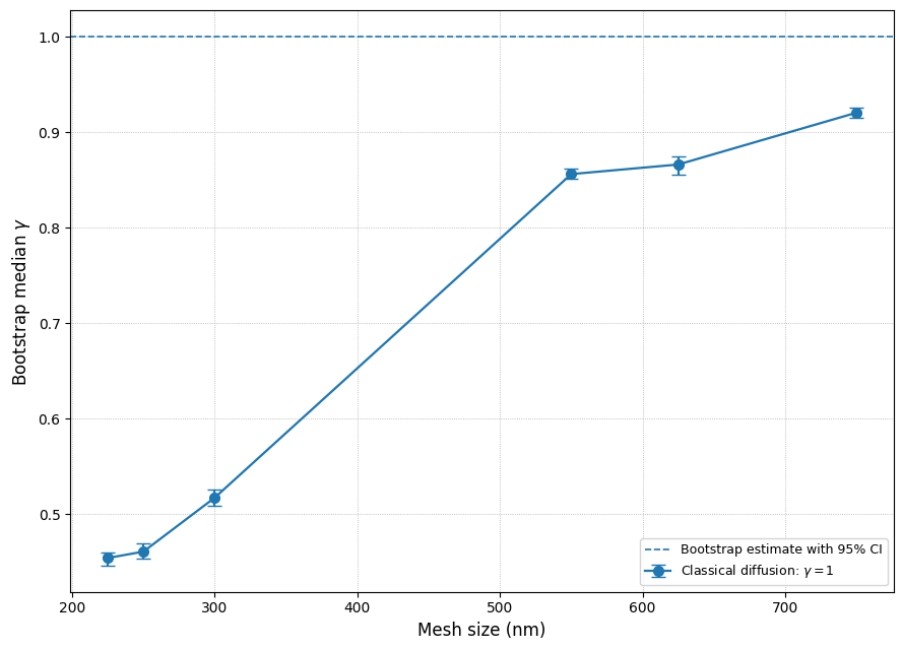
Figure 5: Uncertainty of the empirical scaling exponent due to bootstrap at trajectory level.
Note: Each mesh size provides medians 𝛾∗ = {0.453919,0.460630,0.517128,0.855996,0.866041,0.920303} and empirical 95% intervals; the uncertainty is an estimate of the variability due to sampling the trajectories without assuming independence between lag points. Ensemble estimates are similar to the ones obtained by bootstraping at the trajectory level. The empirical intervals are used to provide uncertainty information, but not assuming that the multiple lag dependent MSD points are independent. The sensitivity of the exponent estimates to fitting-window selection is shown in Figure 6.
Window Dependence
Figure 6: Empirical anomalous-diffusion exponent sensitivity to the fitting-window.
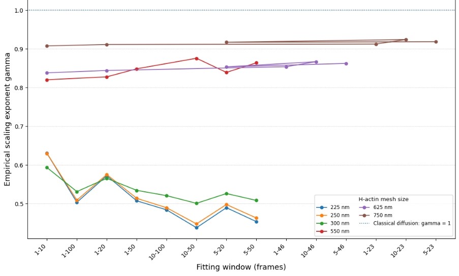
Figure 6: Eight admissible log-log fitting windows per mesh condition quantify the dependence of γ on lag selection; the observed ranges are 0.437679 − 0.630110,0.447543 − 0.629660,0.500728 − 0.593273, 0.820177 − 0.87570, 0.838106 − 0.866882 and 0.907685 − 0.924144 for m = {225, 250, 300, 550, 625, 750} nm. The results of the window-sensitivity analysis indicate that the window-size conditions with smaller meshes are more sensitive to the choice of lag regime. The final value is therefore not only of course based on an objective fitting procedure, but also based on a subjective selection.
Mesh-size trend
The empirical trend is strongly monotone across the six conditions, with slope 0.00099 nm−1 R2 = 0.959955, p = 0.00061, N = 6 This relationship is very empirical, but not a causative law.
Classical diffusion comparison
All the exponents measured are found to be less than γ<1, while for classical diffusive scaling γ=1 is found. The 225-nm condition is the farthest off from the classical limit while the 750-nm condition is the closest to the classical limit.
Interpretation of α
It is not α that is the empirical exponent γ. Data can be released with a unique calibrated model-to-MSD map, if a certain propagator and observation definition are used, leading to an α-dependent scaling. No numerical estimate of α is given, therefore.
Spatial and reaction parameters
The existing scalar MSD measurements are not sensitive to each other's β, κ and λ. The modal transport term includes the two parameters: the spectral parameter β and the transport coefficient κ. The value of the parameter λ represents an effective removal/relaxation contribution that needs to be explicitly modeled describing mass balance.
Theoretical identifiability
The following rank condition, rank 𝐷𝐹(𝜃∗) = 4, is still a mathematically proven condition for any guaranteed continuously differentiable four-parameter observation map. It is not a statement that this is the case with the present experiment; it is just an assumption that it does.
Parameter-estimation status
There are no reliable numerical values of α, β, κ or λ reported. It is a methodological, not computational reason, because the trajectory archive released does not contain the necessary calibration and the necessary information about the model (inverse map) for the following reasons. Figure 7 compares the observed MSD curves with the empirical power-law fits over the selected windows.
Model-data compatibility
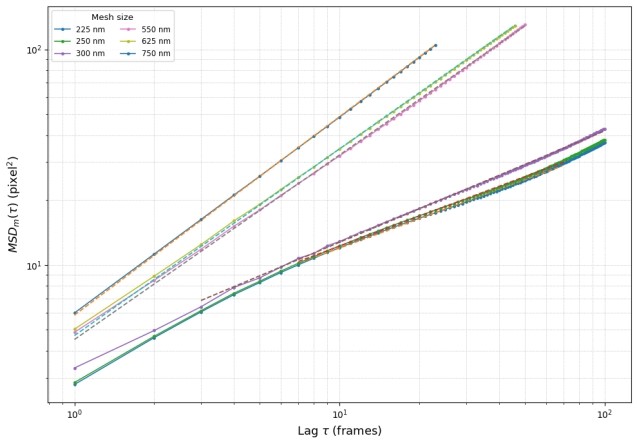
Figure 7: Experimental MSD and objective-window empirical scaling representation.
Note: For each mesh size m = 225, 250, 300, 550, 625 , and 750 nm, the measured MSDm(τ) is compared with Cm τγm over the selected windows 7– 69, 7– 72, 3– 100, 1– 50, 1– 46, and 1– 23 frames, respectively. The corresponding exponents are 0.453412, 0.460879, 0.516736, 0.856105, 0.866278, and 0.920213. The plot represents empirical finite-window scaling and does not provide estimates of α, β, κ, or λ.
Residual and Empirical Fits
The corresponding logarithmic residual patterns are shown in Figure 8.
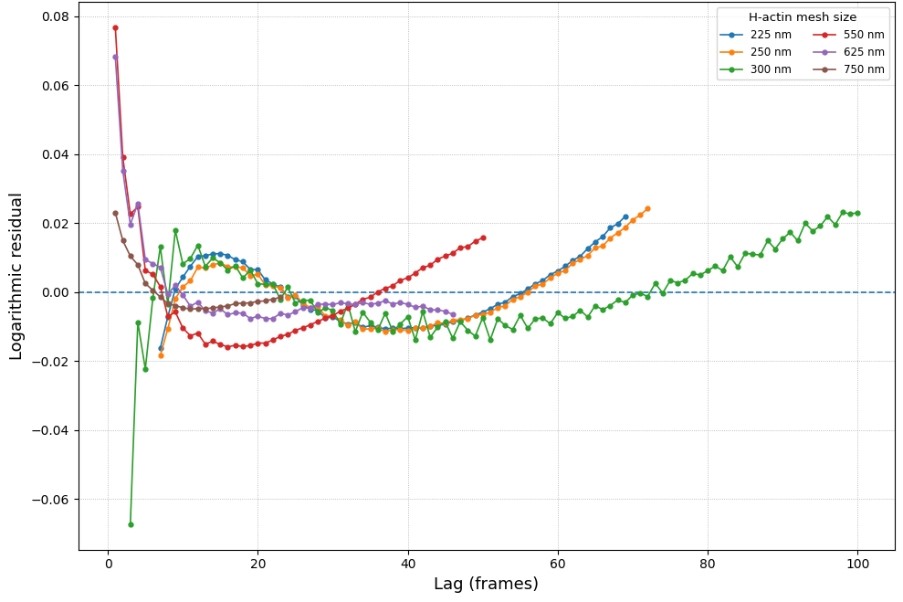
Figure 8: Residual structure of the objective-window empirical scaling fits.
Note: For mesh sizes m = 225, 250, 300, 550, 625 , and 750 nm, the logarithmic residuals rm(τ) = log[MSDm(τ)] − log[Cm τγm] are evaluated over the selected windows 7– 69, 7– 72, 3– 100, 1– 50, 1– 46, and 1– 23 frames, respectively. The residuals describe departures from the empirical power-law fits; they are not residuals from a fitted fractional PDE.
Numerical Validation of The Results and Error Metrics
Validation of the MSD representation of the model is done on the objective lag windows by comparing the model outputs with the residuals by means of error metrics and by computing the log-log coefficient of determination. Let yi be the MSD value observed and ŷi the power-law prediction for the empirical MSD. The Root mean square error (RMSE) is given by:
The mean of the squared errors between the data and the model for the lags used here is the temporal mean-squared error (TMSE).
Goodness of fit is measured as:
For the log-log fit, define 𝑧𝑖 = 𝑙𝑜𝑔(𝑀𝑆𝐷𝑖), and let 𝑧𝑖 denote the fitted 𝑙𝑜𝑔 − 𝑀𝑆𝐷 value. The six objective windows contain 346 lag points in total. The linear-scale TMSE is 0.169075 𝑝𝑖𝑥𝑒𝑙⁴ and the linear-scale RMSE is 0.411187 𝑝𝑖𝑥𝑒𝑙² . The log-scale TMSE is 1.42154 × 10⁻⁴ and the log-scale RMSE is 0.011923. The log-log 𝑅² values for mesh sizes 225, 250, 300, 550, 625, and 750 𝑛𝑚 are 0.999019, 0.998978, 0.999267, 0.999527, 0.999814 , and 0.999962, respectively. These metrics describe empirical power-law fits to the observed MSD; they are not residual metrics for a fractional-PDE fit. Numerical sensitivity-error values are not reported because verified result tables for those outputs were not retained in the frozen archive.
Mathematical validation layer is independent. The functional assumptions that are stated ensure the existence and uniqueness of the solution, the forward stability and parameter continuity are represented in (13) and (14) and the direct sensitivity equations (15-17) are used, while the α direction is treated numerically by a centered finite difference in the verification protocol. Structural-identifiability property is rank 𝐷𝐹(𝜃∗) = 4, in (21) while the singular-value structural-identifiability condition is (23)-(24). This is because the Numerical sensitivity-error values from the benchmark Colab runs were not kept as verified result tables in the frozen archive, and are therefore not given fabricated. The mesh-specific objective-window fit metrics are summarized in Table 4.
| Mesh (nm) | Window (frames) | N | Ensemble γ | Log-log R² | RMSE (pixel²) |
|---|---|---|---|---|---|
| 225 | 7-69 | 63 | 0.453412 | 0.999019 | 0.216538 |
| 250 | 7-72 | 66 | 0.460879 | 0.998978 | 0.247121 |
| 300 | 3-100 | 98 | 0.516736 | 0.999267 | 0.349442 |
| 550 | 1-50 | 50 | 0.856105 | 0.999527 | 0.794277 |
| 625 | 1-46 | 46 | 0.866278 | 0.999814 | 0.386787 |
| 750 | 1-23 | 23 | 0.920213 | 0.999962 | 0.220982 |
Table 4: Empirical validation metrics for the objectively selected MSD scaling windows.
The complete window-selection data and validation calculations are presented in Appendix B, and the computational implementation is provided in Appendix D
The code for the fractional forward solver (Stage 7) and the code for the sensitivity solver (Stage 8) are both numerical verification protocols that are independent. This manuscript does not report invented convergence or sensitivity-error numbers as a result of the fact that their outputs are not independently reported, as verified result tables in the frozen data archive.
Comparisons with Previous Studies
These anomalous-scaling results are in line with the general anomalous-transport literature [2], [6], [20]-[21] and [22]. The framework on the theoretical identifiability is located in the context of fractional identifiability studies [17]-[19] and related structural/practical identifiability literature [13]-[16]. The inverse fractional-diffusion literature cited above [7]- [12], [25]-[28] illustrates the significance of the configuration of the observations and the uniqueness conditions for the models.
LIMITATIONS
The coordinates released are still in pixel units and lag is in frames. No calibration of the physical type was found. The MSD is an observable that is not an observation of PDE state, but rather is derived from a trajectory. There are actually only 6 mesh size conditions available. Last but not least, the present data set is not suitable for an unqualified four parameter mechanistic inversion.
OVERALL INTERPRETATION
The most convincing conclusion from the data is that the MSD scaling of the diffusing fluorescent beads in H-actin networks are sublinear and that the empirical MSD scaling exponent is systematically dependent on the mesh size. The most compelling result, based on the model, is that a fractional diffusion-reaction model can be supported by a well-developed sensitivity and local structural-identifiability analysis, but that a calibrated observation model is needed to obtain quantitative experimental estimates of all four model parameters.
SUMMARY AND CONCLUSION
Summary
In this work, an experimental and mathematical framework was set up for anomalous transport in H-actin networks, with the possibility of tracking this transport. Six major trajectory datasets were used in the MSD pipeline and the integrity of the datasets was confirmed by the structural audits. Objective scaling analysis yielded sublinear exponents that were consistent across the six different mesh-size conditions and bootstrap resampling at the trajectory level provided an estimate of the uncertainty of the exponents.
Principal Findings
The empirical scaling exponents ranged from 0.453412 at 225 nm to 0.920213 at 750 nm. The values increased monotonically with mesh size, with slope 0.00099 nm⁻¹, R²=0.959955, and p=0.00061. The bootstrap medians were not far from the ensemble estimates.
MATHEMATICAL CONTRIBUTION
A local rank-based structural-identifiability theorem, together with sensitivity equations and a Caputo temporal derivative and a spectral fractional spatial operator, were used to formulate a fractional diffusion-reaction framework. The analysis separates analytically the theoretical from the actual experimental recovery.
FINAL CONCLUSION
The results presented here confirm the existence of an anomalous-transport effect in the trajectories of fluorescent beads in H-actin networks, which can be reproduced, and offer a rigorous mathematical framework for studying fractional diffusion-reaction mechanisms. The complete window-selection data and validation calculations are presented in Appendix B, and the computational implementation is provided in Appendix D.
REFERENCES
- Kilbas AA, Srivastava HM, Trujillo JJ. Theory and Applications of Fractional Differential Equations. Amsterdam: Elsevier; 2006. [Google Scholar]
- Metzler R, Klafter J. Boundary value problems for fractional diffusion equations. Physica A. 2000;278(1-2):107-125. [Crossref] [Google Scholar]
- Li X, Xu C. A space-time spectral method for the time fractional diffusion equation. SIAM J Numer Anal. 2009;47(3):2108-2131. [Crossref] [Google Scholar]
- Lin Y, Xu C. Finite difference/spectral approximations for the time-fractional diffusion equation. J Comput Phys. 2007;225(2):1533-1552. [Crossref] [Google Scholar]
- Zhang Y, Xu X. Inverse source problem for a fractional diffusion equation. Inverse Problems. 2011;27(3):035010. [Crossref] [Google Scholar]
- Nazarian P, Haeri M, Tavazoei MS. Identifiability of fractional order systems using input output frequency contents. ISA Trans. 2010;49(2):207-214. [Crossref] [Google Scholar] [PubMed]
- Aghdam TS, Alavi SMM, Saif M. Structural identifiability of impedance spectroscopy fractional-order equivalent circuit models with two constant phase elements. Automatica. 2022;144:110463. [Crossref] [Google Scholar]
- Varalda A, Pequito S. Structural identifiability in fractional-order networks. IFAC J Syst Control. 2026;35:100397. [Crossref] [Google Scholar]
- Schirripa Spagnolo C, Luin S. Trajectory analysis in single-particle tracking: From mean squared displacement to machine learning approaches. Int J Mol Sci. 2024;25(16):8660. [Crossref] [Google Scholar] [PubMed]
- Simon F, Weiss LE, van Teeffelen S. A guide to single-particle tracking. Nat Rev Methods Primers. 2024;4:66. [Crossref] [Google Scholar]
- Granik N, Weiss LE, Nehme E, Levin M, Chein M, Perlson E, et al. Single-particle diffusion characterization by deep learning. Biophys J. 2019;117(2):185-192. [Crossref] [Google Scholar] [PubMed]
- McLean W. Regularity of solutions to a time-fractional diffusion equation. ANZIAM J. 2010;52(2):123-138. [Crossref] [Google Scholar]
- Yan XB, Wei T. Identifying a fractional order and a time-dependent coefficient in a time-fractional diffusion wave equation. J Comput Appl Math. 2023;424:114995. [Crossref] [Google Scholar]
- Jing X, Jia J, Song X. Simultaneous uniqueness identification of the fractional order and diffusion coefficient in a time-fractional diffusion equation. Appl Math Lett. 2025;162:109386. [Crossref] [Google Scholar]
- Chis OT, Banga JR, Balsa-Canto E. Structural identifiability of systems biology models: A critical comparison of methods. PLoS One. 2011;6(11):e27755. [Crossref] [Google Scholar] [PubMed]
- Villaverde AF, Banga JR. Investigating the effect of model parameterization on parameter estimation and identifiability. Bioinformatics. 2015;31(5):835-844. [Crossref] [Google Scholar]
- Jin B, Rundell W. An inverse problem for a one-dimensional time-fractional diffusion problem. Inverse Problems. 2012;28(7):075010. [Crossref] [Google Scholar]
- Li G, Wang Z, Jia X, Zhang Y. An inverse problem of determining the fractional order in the TFDE using the measurement at one space-time point. Fract Calc Appl Anal. 2023;26:1770-1785. [Crossref] [Google Scholar]
- Li YB, Zhou Z. Recovering the potential and order in one-dimensional time-fractional diffusion with unknown initial condition and source. Inverse Problems. 2021;37(10):105009. [Crossref] [Google Scholar]
- Villaverde AF, Barreiro A, Papachristodoulou A. Structural identifiability of dynamic systems biology models. PLoS Comput Biol. 2016;12(10):e1005153. [Crossref] [Google Scholar] [PubMed]
- Heinrich M, Rosenblatt M, Wieland FG, Stigter H, Timmer J. On structural and practical identifiability: Current status and update of results. Curr Opin Syst Biol. 2025;41:100546. [Crossref] [Google Scholar]
- Wang Z, et al. An inverse problem of determining the parameters in diffusion equations by using fractional physics-informed neural networks. Appl Numer Math. 2025;208:189-213. [Crossref] [Google Scholar]
- Lischke A, Pang G, Gulian M, Song F, Glusa C, Zheng X, et al. What is the fractional Laplacian? A comparative review with new results. J Comput Phys. 2020;404:109009. [Crossref] [Google Scholar]
- Amblard F, Maggs AC, Yurke B, Pargellis AN, Leibler S. Subdiffusion and anomalous local viscoelasticity in actin networks. Phys Rev Lett. 1996;77(21):4470-4473. [Crossref] [Google Scholar] [PubMed]
- Stynes M. A survey of the L1 scheme in the discretisation of time-fractional problems. Numer Math Theory Methods Appl. 2022;15(4):1173-1192. [Crossref] [Google Scholar]
- Durdiev DK. Inverse coefficient problem for the time-fractional diffusion equation with Hilfer operator. Math Methods Appl Sci. 2023;46:17469-17484. [Crossref] [Google Scholar]
- Durdiev DK, Turdiev HH. Inverse coefficient problem for a time-fractional wave equation with initial-boundary and integral type overdetermination conditions. Math Methods Appl Sci. 2024;47:5329-5340. [Crossref] [Google Scholar]
- Durdiev DK, Jumaev JJ, Turdiev HH. Inverse problem for determining time dependent coefficient and source functions in a time-fractional diffusion equation. J Math Sci. 2024;289(4):475-486. [Crossref] [Google Scholar]
- Liu Y, Yamamoto M. Uniqueness of inverse source problems for time-fractional diffusion equations with singular functions in time. arXiv:2209.04122. 2022. [Google Scholar]
- Srati M, Oulmelk A, Afraites L, Hadri A, Zaky MA, Hendy AS. Learning primal-dual approach for space-dependent diffusion coefficient identification in fractional diffusion equations. J Comput Phys. 2025;523:113646. [Crossref] [Google Scholar]
- Wang Z, Chen B, Sun H, Liang S. Fractional order system identification using a joint multi-innovation fractional gradient descent algorithm. Sci Rep. 2024;14(1):30802. [Crossref] [Google Scholar] [PubMed]
- Bounouh A, Victor S, Malti R. Convergence analysis of the MISO-OOSRIVCF algorithm for fractional system identification. IFAC-PapersOnLine. 2025;59(37):133-138. [Crossref] [Google Scholar]
- Fardi M, Qasem Al-Omari SK, Araci S. A pseudo-spectral method based on reproducing kernel for solving the time-fractional diffusion-wave equation. Adv Contin Discrete Models. 2022;2022:54. [Crossref] [Google Scholar]
- Dehestani H, Ordokhani Y, Razzaghi M. A spectral approach for time-fractional diffusion and subdiffusion equations in a large interval. Math Model Anal. 2022;27(1):19-40. [Crossref] [Google Scholar]
- Chen Y, Tan X, Huang Y. L2-1σ finite element method for time-fractional diffusion problems with discontinuous coefficients. East Asian J Appl Math. 2023;13(4):813-834. [Crossref] [Google Scholar]
- Li B, Xie X, Yan Y. L1 scheme for solving an inverse problem subject to a fractional diffusion equation. Comput Math Appl. 2023;134:112-123. [Crossref] [Google Scholar]
- Wang L, Stynes M. An α-robust finite difference method for a time-fractional radially symmetric diffusion problem. Comput Math Appl. 2021;97:386-393. [Crossref] [Google Scholar]
- Wang Y, Chen H, Sun T. α-Robust H1-norm convergence analysis of ADI scheme for two-dimensional time-fractional diffusion equation. Appl Numer Math. 2021;168:75-83. [Crossref] [Google Scholar]
- Kumar S, Zeidan D. An efficient Mittag-Leffler kernel approach for time-fractional advection-reaction-diffusion equation. Appl Numer Math. 2021;170:190-207. [Crossref] [Google Scholar]