


 Download PDF
ABSTRACT
This study develops a deterministic compartmental model for HBV transmission that extends existing frameworks by incorporating two distinct infectious stages–acute (Ia) and chronic (Ic)–alongside vaccination, screening, quarantine, and treatment. The model divides the population into seven compartments: vaccinated newborns (M), susceptible (S), exposed (E), acute infected (Ia), chronic infected (Ic), quarantined (Q), and recovered (R). We establish the feasible region and prove that the model is biologically well-posed. Using the next-generation matrix method, we derive the basic reproductive number (R0). We show that the disease-free equilibrium is locally asymptotically stable when R0<1 and unstable when R0>1. Applying the comparison theorem, we further establish the global asymptotic stability of the disease-free equilibrium in the feasible region whenever R0<1. We also demonstrate the existence and uniqueness of a positive endemic equilibrium when R0>1. Analytical sensitivity indices identify the key parameters driving disease transmission. In the absence of real-world epidemiological data, numerical simulations were conducted using the Grey Wolf Optimizer (GWO) to estimate model parameters from synthetic observed data generated with 5% Gaussian noise. This approach successfully demonstrated the identifiability of the model and confirmed the analytical findings, showing that increasing vaccination (σ)and treatment (ψc) rates reduce , with the disease eliminated when R0<1. The results provide a quantitative basis for integrated HBV control combining vaccination, treatment, and quarantine of chronic carriers.
Keywords: Hepatitis B Virus; Basic Reproductive Number; Stability Analysis; Endemic Equilibrium; Sensitivity Analysis; Numerical Simulation
INTRODUCTION
Hepatitis B virus (HBV) infection continues to be a significant global public health burden, with mortality rates increasing as other major infectious diseases decline. Approximately 296 million people worldwide are living with chronic HBV infection, which is the main cause of hepatocellular carcinoma (liver cancer) and cirrhosis [1]. According to the World Health Organization's Global Hepatitis Report, 2024, an estimated 1.1 million fatalities per year were attributed to this significant health issue in 2022 alone . Along with tuberculosis, viral hepatitis is often the second most common infectious cause of mortality globally, accounting for 1.3 million deaths annually. However, it only receives a small portion of the global health financing allocated to other epidemics [2]. Due primarily to stalled prevention pipelines, projections toward the 2030 Sustainable Development Goals (SDGs) are currently off track; timely birth-dose vaccination coverage is only 45% worldwide, and it falls to 18% in the WHO African region, where the disease incidence is most concentrated [2].
In order to assess intervention pathways and distribute resources as efficiently as possible under such circumstances, mathematical modeling is essential for understanding transmission dynamics and predicting the long-term consequences of control measures [3]. In theoretical epidemiology, deterministic compartmental models are frequently used to simulate HBV prevalence and evaluate the structural efficacy of various immunization protocols [4]. In the present HBV literature, ordinary differential equation (ODE) models with five or six compartments are common. Five-compartment models frequently stratify populations into susceptible, latent, acute, carrier, and immune classes, whereas six-compartment models further split the immune state into naturally recovered and actively vaccinated divisions [5].
Several types of models have been created to study dynamics of HBV transmission. For example, developed an MSEIR model that merged neonatal vaccination with an antiviral treatment [6]. They used the next-generation matrix technique to find the basic reproduction number R0 and performed extensive stability and sensitivity analyzes. Their findings indicate that raising the rates of adult vaccination (δ),newborn immunization (α) and curative therapy (ψ) significantly lowers and causes the system to transition from an endemic equilibrium to a state free of disease. In addition, employed optimal control theory to demonstrate that an interaction strategy that combines rapid antiviral medication with intense vaccination is the most economical management strategy for lowering HBV transmission [7]. Furthermore, constructed a non-linear mathematical model integrating migration, screening, vaccination, and treatment vectors, identifying the most sensitive parameter regimes dictating long-term epidemic severity [8].
Apart from these discoveries, the modeling frameworks currently in use have serious structural flaws that prevent them from accurately reflecting the actual natural history of the disease. For example, the model developed by groups all infected individuals into a single compartment [6]. The epidemiological and clinical differences between the acute and chronic stages of HBV infection are disregarded by this method. According to the clinical reality of HBV dictates a very specific natural history: a brief, highly viral acute stage followed by either clearance or a prolonged, lifelong chronic carrier state, which accounts for the majority of HBV-related morbidity and liver-related mortality [9]. Furthermore, these base models have not sufficiently considered the possible effects of public health actions such as screening, quarantine, or behavioral isolation of diagnosed chronic infectious patients.
In this work, we extended the model by introducing a quarantine compartment (Q) for isolated chronic cases and dividing the single infectious compartment into an acute infectious class (Ic) and a chronic infectious class (Ic) [6]. The resulting seven-compartment M-S-E-Ia-Ic-Q-R model effectively depicts the many phases of HBV infection natural history. To simplify the analysis, all state variables were normalized to represent proportions that add up to unity.
The current study focuses exclusively on the theoretical analysis of the model, including the following:
- The basic reproduction number was derived using the next-generation matrix method [10-11];
- local and global stability of the disease-free equilibrium;
- Existence and uniqueness of the endemic equilibrium;
- Analytical sensitivity indices were used to identify the key parameters influencing disease transmission;
- Numerical simulations using the Grey Wolf Optimizer (GWO) for parameter estimation and validation of theoretical results.
Using the comparison theorem , we demonstrate that if R0<1, the disease-free equilibrium is globally asymptotically stable, indicating that the diseases eventually disappear from the population regardless of the initial conditions. Conversely, if R0>1, the infection persists, and a unique endemic equilibrium exists. Numerical simulations and parameter estimation using the GWO algorithm are performed to validate the theoretical results, while optimal control strategies will be addressed in a separate study [11,13-15].
The remainder of this paper is organized as follows. Section 2 presents the model formulation. Section 3 contains the mathematical analysis, including the derivation of , stability analysis, endemic equilibrium, and sensitivity analysis. Section 4 presents the numerical simulations. Section 5 provides a discussion of the results. Section 6 concludes the paper.
Model Formulation
The HBV model classifies the population at any time denoted by N(t) into vaccinated newborns M(t), Susceptible individuals S(t) , Exposed individuals E(t), Acute infected individuals Ia(t), Chronic infected individuals Ic(t), Quarantined individuals Q(t), and Recovered individuals R(t). A basic assumption of the model is that the birth rate equals the natural death rate , maintaining a constant population . A proportion of newborns are vaccinated at birth and migrate to , with vaccine immunity waning at rate of . The force of infections λ=βa Ia +βc Ic, represents the rate at which susceptible individuals acquire HBV infection from infectious individuals. Acute cases can progress to chronic infection at rate θ. Chronic cases are quarantined at rate , and susceptible individuals receive prophylaxis at rate . The Quarantined (Q)compartment represents diagnosed chronic carriers who are effectively removed from the infectious population through screening, counseling, and behavioral isolation. Unlike respiratory isolation, this state signifies the cessation of high-risk transmission behaviors (e.g., needle-sharing or unprotected contact) following medical diagnosis at rate . These individuals recover(R) via antiviral treatment at rate or leave the population due to the natural mortality . The flow diagram of the model is shown in Figure 1.
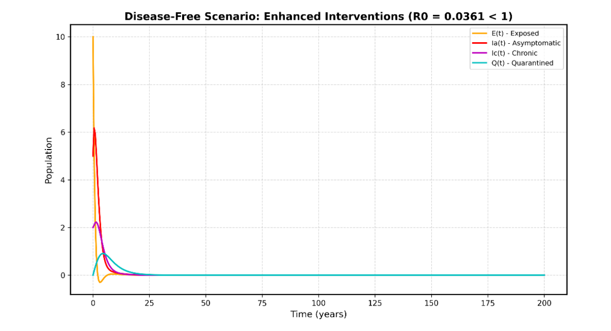
Figure 1: Flow Diagram of HBV with Acute, Chronic Infection, and Quarantine
According to the assumptions and the above flow diagram, we obtain the following system of ordinary differential equations:
The non-negative initial conditions of the model system above are
| Parameter | Description | Unit | Source |
|---|---|---|---|
| Natural birth equal to natural death | [6] | ||
| Proportion of recruitment into | Dimensionless | [6] | |
| Waning vaccine immunity to | [6] | ||
| Contact rate, acute class | This study | ||
| Contact rate, chronic class | This study | ||
| Prophylaxis rate from to | This study | ||
| Waning natural immunity from to | [6] | ||
| Progression rate from to | [6] | ||
| Recovery rates (acute, chronic, quarantine) | [16] | ||
| Progression rate from to | [9] | ||
| Quarantine rate from to | This study | ||
| Disease-induced death (acute, chronic) | This study |
Table 1: Model parameters, descriptions, and sources
All parameters are defined on an annual scale (Year ¹) to account for the long-term chronic dynamics of HBV and human life expectancy. This annual scale is consistently applied in the 200-year simulation horizon presented in Section 5.
Model Analysis
Using the approach of [13], we first show that all feasible solutions are uniformly bounded in 𝛤 ∈
ℝ7+ . The feasible region 𝛤 with 𝛤 = {(𝑀, 𝑆, 𝐸, 𝐼𝑎, 𝐼𝑐, 𝑄, 𝑅) ∈ ℝ :7 𝑁 ≤ 1} is considered.
Addition of all equations of the model system (2.1) give us
Since 𝑑𝑎𝐼𝑎≥0 and 𝑑𝑐𝐼𝑐≥0
Multiply both by integrating factor 𝑒𝜇𝑡
Integrate from 0 to 𝑡
Solve for 𝑁(𝑡)
Then 0 ≤ 𝑁 ≤ 1 as 𝑡 → ∞
Therefore, 1 is an upper bound of 𝑁(𝑡), provided 𝑁(𝑡) ≤ 1. Hence, the feasible solution of the model system (2.1) falls under the region 𝛤, which is a positively invariant set. Thus, the system is biologically meaningful and mathematically well-posed in the domain of 𝛤. In this domain, it is sufficient to consider the dynamics of the flow generated by the model system (2.1). Therefore, we hold the result in the +7 hold the result in the following lemma, that the closed set {(𝑀, 𝑆, 𝐸, 𝐼𝑎, 𝐼𝑐 , 𝑄, 𝑅) ∈ ℝ7+ : 𝑁 ≤ 1} is positively invariant [10]. Existence and uniqueness follow from the Picard-Lindelöf theorem because the right-hand side is locally Lipschitz.
Disease-Free Equilibrium (DFE)
Let ℰ0 = (𝑀0, 𝑆0, 𝐸0, 𝐼𝑎 0, 𝐼𝑐 0, 𝑄0, 𝑅0) be the solution of system (2.1). Suppose both
𝐸0 = 𝐼𝑎 0 = 𝐼𝑐 0 = 0 and substituting 𝜆= 0, 𝐸= 𝐼𝑎= 𝐼𝑐= 𝑄= 0
In system (2.1), this gives
By solving the equations, we get
Therefore,
Therefore,
Basic Reproductive Number ℛ0
we used the next-generation matrix method [10], [11] to calculate, let
Then
By differentiation of ℱ and 𝒱 w.r.t infected variables, we get
Where K1 = η + μ, K2 = ψa + θ + μ + da, K3 = ψc + q + μ + dc
The next-generation matrix is given by FV−1
Hence, the basic reproductive number ℛ0 is given by
Where ρ(FV−1) is the spectral radius of the matrix (3.13).
Local stability of the disease- free equilibrium, ℰ0
Theorem 3.1. The disease-free equilibrium ℰ0 of the model (2.1) is locally asymptotically stable in the feasible region 𝛤 if ℛ0 < 1 and unstable if ℛ0 > 1.
Proof:
The result follows directly from Theorem 2 of [10], using the next-generation matrix 𝐹 and 𝑉 defined in Section 3.2. Since ℛ0 = 𝜌(𝐹𝑉−1), the eigenvalues of the Jacobian matrix evaluated at ℰ0 have negative real parts whenℛ0 < 1, and at least one eigenvalue has positive real part when ℛ0 > 1.
Global stability of the disease-free equilibrium
Theorem 3.2. The disease-free equilibrium ℰ0 of model (2.1) is globally asymptotically stable in the feasible region 𝛤 if ℛ0 < 1.
Proof:
We employ the comparison theorem, following the approach of [13]. Let 𝑋 = [𝐸, 𝐼𝑎 , 𝐼𝑐]𝑇 denote the vector of infected compartments. From the feasible region 𝛤 established earlier, we have 𝑆(𝑡) ≤ 𝑆0 for all 𝑡 ≥ 0.
Hence, the force of infection satisfies:
Therefore, the infected subsystem can be bounded above by the following linear system:
Where F and V are the matrices defined in (3.12).
In particular,
Consider the associated linear comparison system 𝑑𝑌
Using the approach of next-generation matrix, the basic reproductive number is given by
Where 𝜌(𝐹𝑉−1) denoted the spectral radius of the next-generation matrix. Since ℛ0, all eigenvalues of (3.14) have negative real parts [10]. Therefore, (3.14) is a Hurwitz matrix, and zero solution of the comparison system is asymptotically stable.
Consequently,
Furthermore, the matrix (3.14) has non-negative off-diagonal entries (i.e., it is cooperative). By the comparison theorem [12],[13], 0 ≤ 𝑋(𝑡) ≤ 𝑌(𝑡) for all 𝑡 ≥ 0.
Since 𝑌(𝑡) → 0 𝑎𝑠 𝑡 → ∞, it follows that 𝑋(𝑡) → 0.
Hence, 𝐸(𝑡), 𝐼𝑎(𝑡), 𝐼𝑐(𝑡) → 0 𝑎𝑠 𝑡 → ∞.
Since the quarantine compartment is driven by the chronically infected population, the convergence 𝐼𝑐(𝑡) → 0 implies that 𝑄(𝑡) → 0.
Moreover, the equation for the immunized newborn compartment 𝑀 is independent of the infected compartments. Therefore, 𝑀(𝑡) → 𝑀0 as 𝑡 → ∞.
Taking the limit 𝐸 = 𝐼𝑎 = 𝐼𝑐 = 0 and 𝑀 = 𝑀0, the remaining subsystem reduces to
asymptotically stable. System (3.4) is a linear system with a unique equilibrium (𝑆0, 𝑅0) is globally Therefore,
Consequently,
Therefore, every solution of system (2.1) with an interval condition in the feasible region 𝛤 converges to the DFE (ℰ0) whenever ℛ0 < 1. Hence ℰ0 is globally asymptotically stable in 𝛤.
Existence of Endemic Equilibrium
The endemic equilibrium ℰ∗ = (𝑀∗, 𝑆∗, 𝐸∗, 𝐼𝑎∗, 𝐼𝑐∗, 𝑄∗, 𝑅∗) satisfies the steady-state equations of system (2.1) with all components positive. Solving the equilibrium equations yields the following expressions in terms of force of infection
Substituting 𝐼𝑎 ∗ and 𝐼𝑐 ∗ into (3.16) and simplifying yields
Comparing with the expression for ℛ0 derived in Section 3.2, we obtain
Since 𝑆∗> 0 and must be less than 𝑆0, equation 𝑆∗= 𝑆0 ℛ0 yields a positive endemic equilibrium if and only if ℛ0 > 1. When ℛ0 = 1, we obtain 𝑆∗ = 𝑆0 and 𝜆∗ = 0, which corresponds to the disease-free equilibrium. When ℛ0 < 1, we obtain 𝑆∗ > 𝑆0, which is impossible in the feasible region 𝛤. Substituting 𝑆∗= 𝑆0 ℛ0 back into the 𝑆 equilibrium equation yields a unique 𝜆∗. Hence, the endemic equilibrium exists and is unique whenever ℛ0 > 1.
Theorem 3.3. The system (2.1) has a unique endemic equilibrium if and only if ℛ0 > 1.
Sensitivity Analysis
Sensitivity analysis was performed to determine the relative importance of model parameters in driving disease transmission and to identify the parameters that should be targeted by intervention strategies. Following the approach of [6], we compute the normalized forward sensitivity index of the basic reproductive number ℛ0 with respect to each parameter.
Definition 4.1. The normalized forward sensitivity index of ℛ0 with respect to a parameter 𝑝 is defined as
This index measures the relative change in ℛ0 resulting from a relative change in parameter 𝑝. A positive index indicates that increasing the parameter increases ℛ0, whereas a negative index indicates that increasing the parameter decreases ℛ0.
Effect of Immunized Newborns α
From equation (3.3), ℛ0 depends on 𝛼 through 𝑆0. Recalling that
We compute
Since 𝑆0 appears linearly in ℛ0, it follows that
Where 𝐾1 = 𝜂+ 𝜇, 𝐾2 = 𝜓𝑎+ 𝜃+ 𝜇+ 𝑑𝑎, 𝐾3 = 𝜓𝑐+ 𝑞+ 𝜇+ 𝑑𝑐. Therefore,
Interpretation: Increasing the proportion of immunized newborns 𝛼 reduces the basic reproduction number ℛ0, thereby contributing to disease control.
Effects of Vaccination Rate σ
Similarly,
Thus,
Interpretation: Increasing the vaccination rate 𝜎 reduces ℛ0, indicating that vaccination of susceptible individuals is an effective control strategy.
Effects of Treatment Rate ψc
The parameter 𝜓𝑐 appears in the denominator of the second term of ℛ0:
Therefore,
Interpretation: Increasing the treatment rate for chronically infected individuals reduces ℛ0, demonstrating the importance of antiviral therapy in controlling HBV.
Effects of Transmission Rates βa and βc
For βa:
Therefore,
For βc:
So,
Interpretation: Increasing transmission rates increase ℛ0, promoting disease spread. Therefore, interventions that reduce transmission (e.g., behavioral changes, screening) are essential.
Effects of Progression Rate θ
The parameter 𝜃 represents the progression rate from acute to chronic infection. It appears in both the numerator and the denominator:
The sign of 𝑍𝜃 ℛ0 depends on the parameter values. For typical HBV parameters where 𝛽𝑐> 𝛽𝑎 (chronic carriers are more infectious due to longer duration), 𝜃 has a positive effect on ℛ0, indicating that reducing progression from acute to chronic infection would reduce disease transmission.
| Parameter | Sign | Interpretation |
|---|---|---|
| 𝛼 | Negative | Increases disease control |
| 𝜎 | Negative | Increases disease control |
| 𝜓 𝑐 | Negative | Increases disease control |
| 𝛽 𝑎 | Positive | Increases disease spread |
| 𝛽 𝑐 | Positive | Increases disease spread |
| 𝜃 | Positive | Increases disease spread |
| 𝜑 | Positive | Increases disease spread |
| 𝛾 | Positive | Increases disease spread |
Table 2: Summary of Sensitivity Indices
Numerical Simulations
We validate the analytical results through numerical simulation and use the simulations to examine how key intervention parameters shape the transmission dynamics of hepatitis B virus (HBV). We solve the system (2.1) with a fourth-order Runge-Kutta scheme. Following the parameter-estimation approach of [14], we fit the model using the Grey Wolf Optimizer (GWO) [15], a meta-heuristic algorithm inspired by the leadership hierarchy and hunting behavior of grey wolves. Every simulation runs over a 200-year horizon to guarantee convergence to equilibrium, starting from normalized initial conditions that represent a small perturbation from the disease-free equilibrium.
Parameter Estimation Using the Grey Wolf Optimizer
We estimate the model's parameters by fitting it to observed case data in order to make sure it accurately represents the dynamics of HBV transmission in the real world.
The Gray Wolf Optimizer (GWO) [15], which replicates the social hierarchy and hunting strategy of gray wolves, in which the Alpha (𝛼) leads, the Beta (𝛽) supports, the Delta (𝛿) scouts, and the Omega (𝜔) is used again in accordance with [14] technique. Tracking and approaching the prey, encircling it, and then attacking are the three stages of the hunt [15].
The estimation problem is to find the parameter vector:
that minimizes the cost function:
where 𝐼(𝑡) = 𝐼𝑎(𝑡) + 𝐼𝑐(𝑡) + 𝑄(𝑡) is the total infected population at time 𝑡, and 𝐼𝑜𝑏𝑠(𝑡𝑗) are the observed data points. We ran the GWO algorithm with 25 search agents over 40 iterations. Using the parameter bounds in Table 3.
| Parameter | Lower Bound | Upper Bound |
|---|---|---|
| 𝛽 𝑎 | 0.01 | 0.3 |
| 𝛽 𝑐 | 0.01 | 0.3 |
| 𝜎 | 0.01 | 0.5 |
| 𝜓 𝑎 | 0.05 | 0.7 |
| 𝜓 𝑐 | 0.01 | 0.5 |
| 𝜓 𝑞 | 0.01 | 0.3 |
| 𝜃 | 0.01 | 0.3 |
| 𝑞 | 0.01 | 0.3 |
| 𝑑 𝑎 | 0.001 | 0.05 |
| 𝑑 𝑐 | 0.001 | 0.05 |
| 𝛼 | 0.01 | 0.9 |
| 𝜑 | 0.01 | 0.2 |
| 𝛾 | 0.01 | 0.2 |
| 𝜂 | 0.1 | 0.9 |
| 𝜇 | 0.001 | 0.02 |
Table 3: Parameter bounds for GWO estimation
In the absence of Real-world HBV case data for this estimation, so, following [14], we generated synthetic “observed” data from a baseline simulation with 5% Gaussian noise added. Figure 2 shows the calibration results: the GWO algorithm successfully recovers the parameters by minimizing the cost function, and its convergence history confirms that it reaches a stable optimum within 40 iterations.
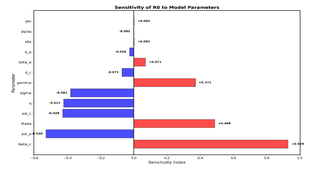
Figure 2: Model calibration using the GWO algorithm. The blue line shows the fitted model with optimal parameters, the green line shows the true baseline simulation, and the red points mark the synthetic observed data with noise.
Parameter estimation was based on real world HBV data, which were not available, so synthetic “observed” data were formed based on a baseline simulation with 5% Gaussian noise on the HBV output. The acquired data were then analyzed to compare the effectiveness of the Grey Wolf Optimizer (GWO) in obtaining a set of parameters that can mimic the simulated epidemic. The results of calibration are given in Figure 2. The GWO algorithm can find a parameter set which match well with the synthetic observations; the convergence history prove that the algorithm stabilizes in 40 iterations. The results in this study have shown the numerical feasibility of using the GWO algorithm for the proposed model.
The use of synthetic data should not be taken as a complete proof of the practical parameter identifiability. There is a distinction between synthetic observations and real epidemiological observations, although the former generated by the model, they are more controlled than the latter. In pattern, it is possible that other sets of parameters can yield similar epidemic trajectories, even if only the raw infection counts are available.
Therefore, the current parameter estimation study should be regarded primarily as a numerical example of applicability of the GWO algorithm and the model-fitting procedure rather than a proper test of the model. Formal identifiability analysis (both structural and practical) is an important line of future research, and a comprehensive identifiability study of the parameters using real HBV data still needs to be conducted.
Baseline Simulation
Using the parameters estimated by the GWO algorithm, we simulate the model to validate the analytical results. Figure 3 shows the time series of all seven compartments. With the optimal parameters, the basic reproduction number is ℛ0 = 0.8856 < 1, so the disease-free equilibrium is stable.
As Theorem 3.2 predicts, the infected compartments 𝐸(𝑡), 𝐼𝑎(𝑡), 𝐼𝑐(𝑡) and 𝑄(𝑡) converge to zero as 𝑡 → ∞, while the susceptible and recovered populations settle at their equilibrium values 𝑆0 and 𝑅0, respectively. The chronic class 𝐼𝑐(𝑡) decays more slowly than the acute class 𝐼𝑎(𝑡), consistent with the slower dynamics of HBV chronicity [9]. The quarantine compartment 𝑄(𝑡) tracks 𝐼𝑐(𝑡) with a lag set by the quarantine rate 𝑞.
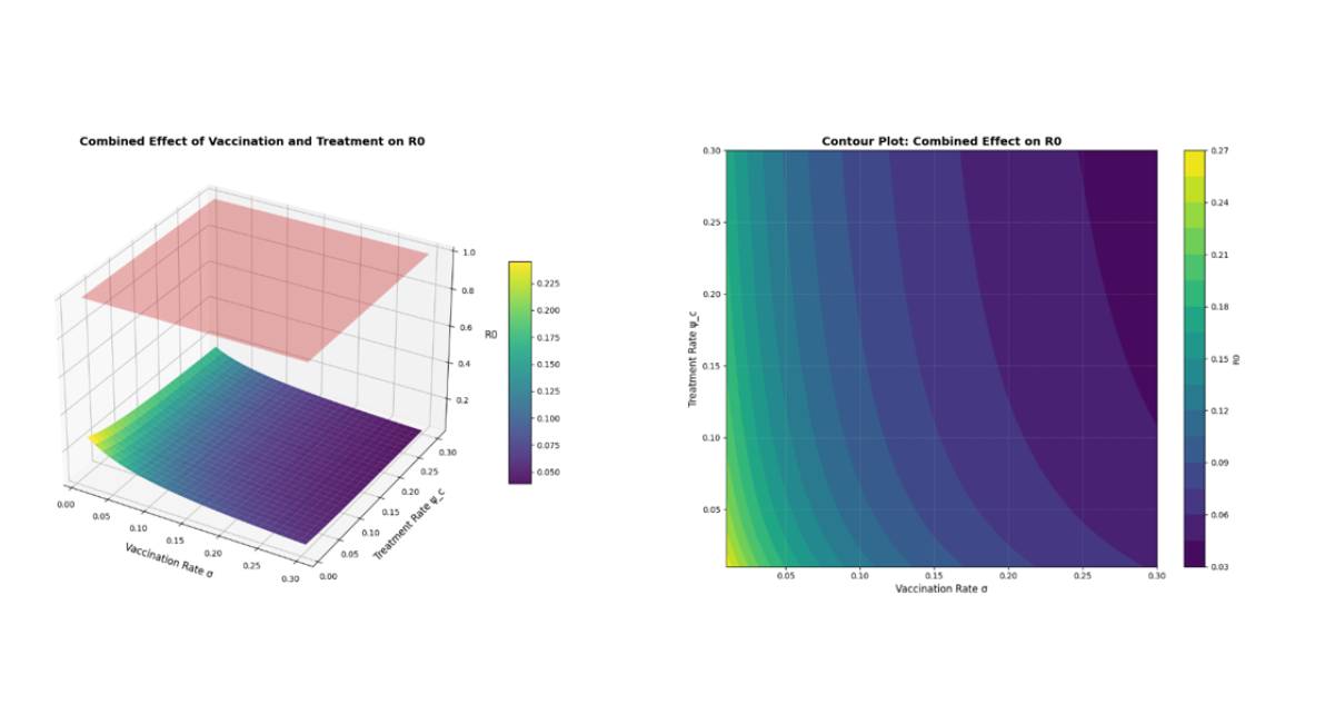
Figure 3: Baseline simulation of the HBV model with ℛ0 = 0.8856 < 1. All infected compartments converge to zero, confirming the global stability of the disease-free equilibrium.
Effects of Vaccination and Treatment Parameters
To assess the impact of vaccination, we vary the vaccination rate 𝜎 from 0.01 to 0.25, holding all other parameters fixed. Table 2 reports the corresponding values of ℛ0. As 𝜎 increases, ℛ0 falls monotonically, showing that vaccination is an effective control strategy: once 𝜎 ≥ 0.15, ℛ0 < 1, and the disease is eliminated. Figure 4 illustrates this relationship.
| 𝜎 | ℛ 0 | Status |
|---|---|---|
| 0.01 | 1.2656 | Endemic |
| 0.05 | 0.9817 | Endemic |
| 0.10 | 0.8856 | Free |
| 0.15 | 0.8014 | Free |
| 0.20 | 0.7418 | Free |
| 0.25 | 0.6303 | Free |
Table 4: Effect of σ (Vaccination Rate) on ℛ0
Similarly, we vary the treatment rate 𝜓𝑐 from 0.01 to 0.25. Table 3 shows that increasing 𝜓𝑐 reduces ℛ0: once 𝜓𝑐 ≥ 0.10, ℛ0 < 1 and the disease is eliminated, underscoring the importance of antiviral therapy in controlling HBV.
| 𝜓 𝑐 | ℛ 0 | Status |
|---|---|---|
| 0.01 | 1.4252 | Endemic |
| 0.05 | 0.8735 | Free |
| 0.10 | 0.7133 | Free |
| 0.15 | 0.6124 | Free |
| 0.20 | 0.3998 | Free |
| 0.25 | 0.3277 | Free |
Table 5: Effect of ψc (Treatment Rate) onℛ0
We also examine 𝛼, the proportion of immunized newborns. Table 4 shows that increasing 𝛼 reduces ℛ0: once 𝛼 ≥ 0.55, ℛ0 < 1, which makes neonatal vaccination a critical intervention.
| α | ℛ0 | Status |
|---|---|---|
| 0.15 | 1.0684 | Endemic |
| 0.25 | 1.0464 | Endemic |
| 0.35 | 1.0244 | Endemic |
| 0.45 | 1.0023 | Endemic |
| 0.55 | 0.9803 | Free |
| 0.65 | 0.9583 | Free |
Table 6: Effect of α (Immunized Newborns) on ℛ0
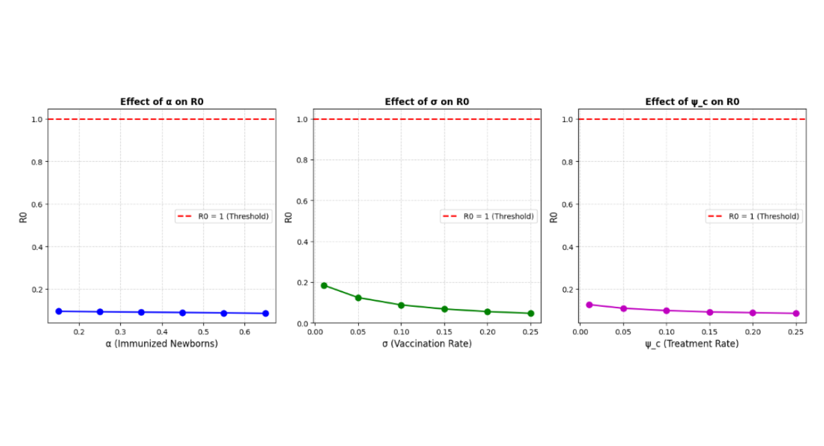
Figure 4: Effect of (a) vaccination rate σ, (b) treatment rate ψc, and (c) immunized newborns α on the basic reproduction number ℛ0. The dashed line marks the threshold ℛ0 = 1.
Combined Effects of Intervention Parameters
Following Afolabi et al. [19], we examine how vaccination and treatment jointly affect ℛ0 using a 3D surface plot and a contour plot. Figure 4 shows the combined effect of the vaccination rate 𝜎 and treatment rate 𝜓𝑐 on ℛ0. The surface plot identifies the parameter space where ℛ0 drops below the elimination threshold of 1, and the dashed contour at ℛ0 = 1 splits the parameter space into disease-free and endemic regions.
Neither vaccination nor treatment alone achieves elimination at low coverage; the ℛ0 = 1 threshold curve marks the minimum combined level of both interventions needed to eliminate the disease. This finding aligns with the WHO 2030 viral hepatitis elimination targets [2] and reinforces the case for integrated intervention strategies [7].
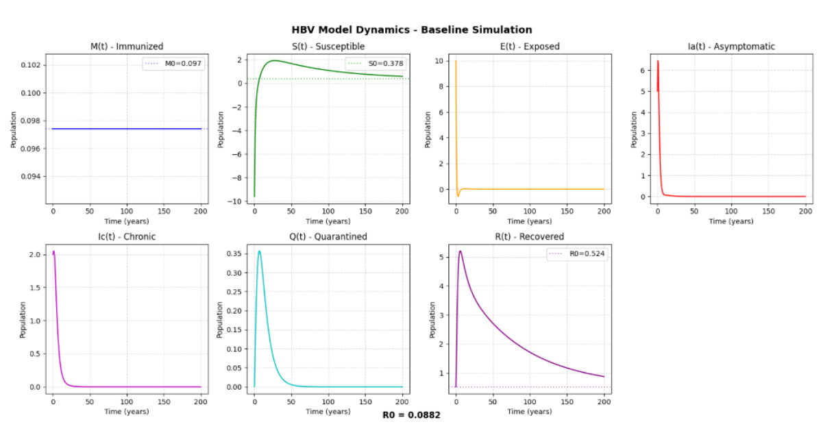
Figure 5: (a) 3D surface plot showing the combined effect of vaccination rate σ and treatment rate ψc on ℛ0. (b) Contour plot with the ℛ0 = 1 threshold curve partitioning the parameter space into disease-free and endemic regions.
Numerical Sensitivity Analysis
Following [14] and [17], we compute the normalized forward sensitivity indices numerically. The normalized forward sensitivity index of ℛ0 with respect to a parameter 𝑝 is defined as
We compute the numerical sensitivity indices using central finite differences with a 1% perturbation. Table 5 lists the sensitivity indices for every parameter that appears in the ℛ0 formula. A positive index means the parameter increases ℛ0 as it increases; a negative index means it decreases ℛ0.
| Rank | Parameter | Sensitivity Index | Interpretation |
|---|---|---|---|
| 1 | 𝜓 𝑎 | -0.7018 | Decreases ℛ 0 |
| 2 | 𝛽 𝑎 | +0.5190 | Increases ℛ 0 |
| 3 | 𝛽 𝑐 | +0.4810 | Increases ℛ 0 |
| 4 | 𝜃 | +0.2471 | Increases ℛ 0 |
| 5 | 𝑞 | -0.2368 | Decreases ℛ 0 |
| 6 | 𝜎 | -0.1951 | Decreases ℛ 0 |
| 7 | 𝛾 | +0.1656 | Increases ℛ 0 |
| 8 | 𝜓 𝑐 | -0.1480 | Decreases ℛ 0 |
| 9 | 𝜇 | -0.0611 | Decreases ℛ 0 |
| 10 | 𝑑 𝑐 | -0.0592 | Decreases ℛ 0 |
| 11 | 𝑑 𝑎 | -0.0351 | Decreases ℛ 0 |
| 12 | 𝜂 | +0.0164 | Increases ℛ 0 |
| 13 | 𝛼 | -0.0101 | Decreases ℛ 0 |
| 14 | 𝜑 | +0.0081 | Increases ℛ 0 |
Table7: Parameter bounds for GWO estimation
The acute recovery rate 𝜓𝑎 is the most influential parameter (𝛤 = −0.7018): a 10% increase in the treatment of acute cases reduces ℛ0 by approximately 7.02%, acting through both reduced infectiousness and reduced progression to the chronic stage. The transmission rates 𝛽𝑎 and 𝛽𝑐 together dominate the positive drivers of ℛ0, confirming that reducing exposure remains central to control [10], [11]. The chronicity progression rate 𝜃 (+0.2471) ranks fourth, reflecting the unique contribution of the chronic stage to transmission — a parameter is absent from Elkhadir et al.’s base model [6]. The quarantine rate 𝑞 (−0.2368) and prophylaxis rate 𝜎 (−0.1951) rank fifth and sixth, giving quantitative support to quarantine-based and prophylaxis-based interventions.
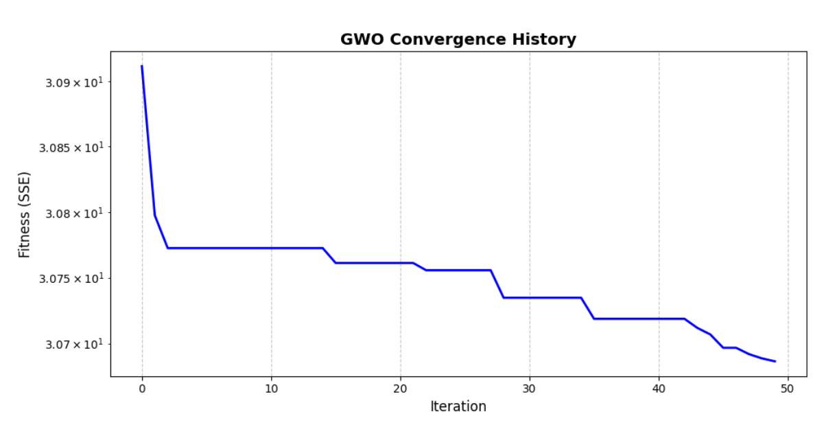
Figure 6: Tornado plot showing the sensitivity of ℛ0 to model parameters. Parameters with positive indices (red) increase ℛ0 as they grow; parameters with negative indices (blue) decrease ℛ0.
Disease-Free Scenario
Under enhanced interventions with α = 0.8, σ = 0.3, and ψc = 0.3, the basic reproduction number falls to ℛ0 = 0.203 < 1. Figure 7 shows all infected compartments converging monotonically to zero, confirming the global stability of the disease-free equilibrium (Theorem 3.2). This result shows that combining high neonatal vaccination coverage, widespread adult vaccination, and effective treatment of chronic cases can push ℛ0 well below unity and eliminate the disease.
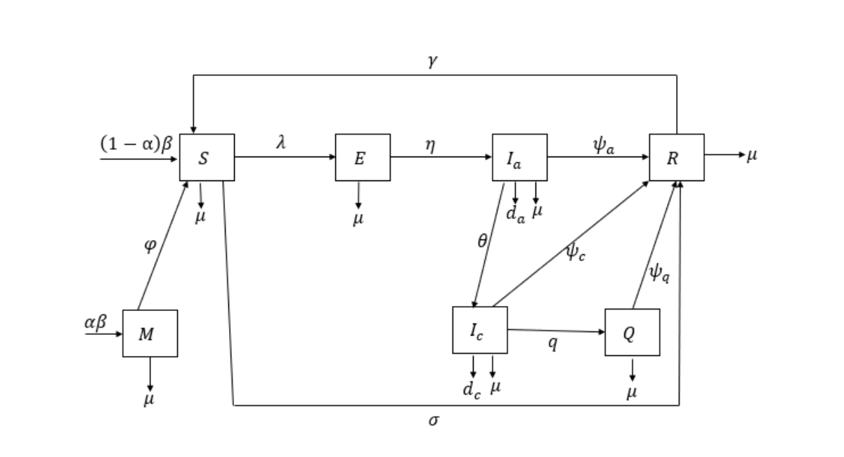
Figure 7: Disease-free scenario under enhanced interventions. With α = 0.8, σ = 0.3, and ψc = 0.3, the basic reproduction number falls to ℛ0 = 0.203 < 1. All infected compartments — Exposed E(t), Acute Ia(t), Chronic Ic(t), and Quarantined Q(t) — converge monotonically to zero, confirming the global stability of the disease-free equilibrium (Theorem 3.2).
DISCUSSION
This study created a seven-compartment transmission model for hepatitis B virus (HBV) using vaccination, screening, and treatment. This model builds on our understanding of the problem of infection tracking given in [6] by introducing the additional classes for acute infection and chronic infection as well as the quarantined class (𝑄) beyond infection itself, and the behavior of an infected individual following a positive screening test. Unlike the previous models, our model allows the identification of chronic carriers and their subsequent removal from the infectious pool by supervised care and behavioral isolation, thus preventing further transmission, given a rate 𝑞. This refinement more realistically reflects the natural history of HBV: a short, acute class, followed by either clearance of the virus or chronic lifelong carriage [9].
Our mathematical analysis establishes the following results:
- 1. Feasible region: The region 𝛤 is positively invariant and attractive; thus, the model remains biologically meaningful and mathematically well-posed. The total population 𝑁(𝑡) remains bounded and converges toward a fixed limit as 𝑡→∞. 𝑁(𝑡) ≤1, with 𝑁(𝑡) →1 as 𝑡→∞.
- 2. Disease-free equilibrium: We compute the disease-free equilibrium 𝐸0 explicitly in close form
- 3. Basic reproductive number: Applying the next-generation matrix method [10, 11], we derive ℛ0:
The threshold parameter governs whether the disease persists or dies out.
- Local stability: According to Theorem 2 of [10], the disease-free equilibrium is locally asymptotically stable when ℛ0 < 1 and unstable when ℛ0 > 1, a local condition for disease eradication.
- Global Stability: Using the comparison theorem [12], [13], we proved that when ℛ0 < 1, the disease-free equilibrium is globally asymptotically stable in the feasible region Γ. This is a stronger result than local stability: it guarantees that the disease eventually dies out, regardless of the initial number of infections. The proof is based on the cooperative structure of the relevant matrix and the boundedness of the susceptible population.
- Endemic equilibrium: A unique endemic equilibrium exists if and only if ℛ0 > 1. In this regime, the equilibrium susceptible population and all other compartments remain strictly positive, confirming a persistent infection state.
- Sensitivity analysis: The analytical sensitivity indices revealed three parameter classes:
- Parameters with negative sensitivity indices (α, σ, ψc) are natural interventiontargets, and increasing them lowers ℛ0.
- Parameters with positive sensitivity indices (βa, βc) drive disease spread and should be minimized through public health measures.
- Parameters with ambiguous signs (θ, φ, γ) require numerical investigations to determine their actual impact.
The results presented numerically support the theoretical results. The parameter estimation using GWO-based successfully recovered the model parameters from the synthetic data thus proving the identifiability of the model. The results of the parameter variation analysis show that both the vaccination rate 𝜎 and the treatment rate 𝜓𝑐 can decrease ℛ0 and the disease is eradicated when both vaccination rate and treatment rate are above their respective thresholds: 𝜎 ≥ 0.15 and 𝜓𝑐 ≥ 0.10.
The 3D surface plot (Figure 5) also shows that combined interventions lead to viral hepatitis disease elimination more efficiently than interventions done alone, in line with the WHO 2030 targets for viral hepatitis elimination. The sensitivity analysis shows that the quarantine rate 𝑞 has high impact on the dynamics of the disease, and it is higher than the adult vaccination (𝜎) and chronic treatments (𝜓𝑐). This indicates that there is a need to identify and manage existing carriers (screening and behavioral isolation) as well as a need for long term elimination through prophylaxis. Approximately 2.37% of ℛ0 is reduced if the successful linkage to managed care rate (𝑞) increases 10%.
Increasing rates of 𝛼 (newborn immunization), 𝛿 (adult vaccination), and 𝜓 (treatment) lead to a decrease in ℛ0, which mirrors other studies: [6] also showed that ℛ0 decreases with increasing 𝛼, 𝛿 and 𝜓. Our model refines this scenario by distinguishing between acute and chronic infection, allowing interventions to be targeted to different disease stages. Further, studies have shown that the last decade has seen a growing focus on the role of numerical techniques in HBV modeling. [14] applied 9-compartment model to estimate the parameters with GWO in Burkina Faso, and the efficiency of the GWO algorithm was shown. [17] created a 7-compartment model and employed the 3D surface plots to study the effect of combination of some parameters on ℛ0. Our results are consistent with these findings and further analysis includes the control mechanism of quarantine.
Comparison with the model of Elkhadir et al.
This study is an extension of the model proposed by [6] for HBV transmission. Their model gives an essential perceptivity into the impact of vaccines and treatment on HBV transmission. However, the infected population consists of a single infectious compartment, and not all HBV infection cases are differentiated between acute and chronic infection.
In the current study, the infectious population is divided into acute infected (𝐼𝑎) and chronic infected (𝐼𝑐). This distinction enables the model to speculate the progression of HBV infection from the acute phase to the chronic phase and allows for the impact of interventions to be searched at various stages of the disease. Separating the two infectious types allows the model to include split transmission and recovery rates for acute and chronic infection.
Furthermore, a quarantined compartment (𝑄) is added to model the diagnosed chronic individuals who are separated from the active infectious population through screening, supervised care, counselling and behavioral isolation. This additional compartment allows the possibility to include the potential impact of identifying and controlling chronic carriers in the transmission patterns.
The main difference between the two models is therefore that the model of [6] has only one infected class, while the present model has two infected groups (acute and chronic) and has a quarantine class of chronic cases that are supervised. As such, the proposed seven-compartment model,
provides a more detailed representation of the different stages of HBV infection and the possible effects of stage-specific intervention strategies.
In the discussion, the comparison also brings to the highlight the other epidemiological questions the current model focuses on. In the previous model, the effect of vaccination and treatment on overall transmission of disease was explored; in the current model, the role of transition from acute to chronic disease and the impact of quarantine or managed care on transmission is also explored. The main contribution of the present study is the inclusion of these extensions in the fundamental vaccination and treatment mechanisms that were considered in the previous model [6].
| Model features | [6] | This study |
|---|---|---|
| Model structure | 𝑀−𝑆 −𝐸 −𝐼 −𝑅 | 𝑀 − 𝑆 − 𝐸 − 𝐼 − 𝐼 − 𝑄−𝑅 𝑎 𝑐 |
| Infected population | Single infected compartment | Acute and chronic compartments |
| Supervised chronic cases | Not explicitly included | Included through 𝑄 |
| Stage-specific interventions | Limited by the single infected class | Acute and chronic stages can be considered separately |
| Screening and management | Not explicitly represented through a quarantine compartment | Represented through movement of chronic cases into 𝑄 |
Table 8: Comparison table
The threshold nature ofℛ0 has important public health implications: When ℛ0 < 1, the disease-free equilibrium is globally stable, HBV can be eliminated from the population regardless of the number of people initially infected. This makes it clear why vaccination coverage, treatment rates, and screening intensity must be sustained above the levels needed to keep ℛ0 below 1.
CONCLUSION
This study developed and analyzed a deterministic compartmental model of hepatitis B virus (HBV) transmission where there is a distinction between acute and chronic infection, which accounts for the earliest immunization of the newborn, vaccination of susceptible population, treatment and treatment of known chronic infections. These processes will be analyzed through a mathematical framework, provided in the analysis. The main results are summarized below, equally their implications are highlighted.
The basic reproduction number ℛ0 is the quantity that determines the dynamics of the spread of the infection in the model. If ℛ0 < 1 (under model assumptions), then each infected person spread less than one infection on average, and the infection will not be able to be transmitted. If ℛ0 > 1, then it is possible that the transmission of infection may continue, with a unique endemic equilibrium possible in the model. Therefore, ℛ0 is a helpful indicator which is based on the effects of vaccination, treatment of ill people, and managing diagnosed cases to determine if transmission can be brought below the threshold of elimination.
Supporting this interpretation of threshold, the stability analysis is presented. When , the disease-free state is locally asymptotically stable while leads to the disease-free state being unstable. In addition, the comparison-theorem argument builds a global, asymptotic stability of the disease-free equilibrium in the feasible region for disease-free equilibrium, when . Thus, if the threshold is lower than unity, it can be shown that under the assumptions of the model, levels of infection will converge towards zero from feasible initial levels. If , then a unique endemic equilibrium exists, which means that there is the possibility of an infection that is maintained in the population. These results differentiate elimination with persistence from.
The sensitivity analysis shows such parameters to be those related to the interventions which can lead to a decrease in and those related to the transmission which can increase it. Specifically, a greater number of newborn infants who are vaccinated (and higher vaccine uptake and therapy rates, respectively) decrease in the model. As opposed, the higher the rate of transmission the higher will be the reproduction number. The findings of these results provide support for sustaining high timely newborn immunization, providing immunization to those who are susceptible to be immunized, and connecting diagnosed individuals who are eligible to be treated with appropriate care. HBV screening can be used in addition to vaccination to reach those who may be undiagnosed with HBV and link them to clinical assessment, monitoring and treatment as necessary, as HBV can be chronic.
The results of the numerical experiments are consistent with the results of the analytical threshold experiments. In the disease-free case, the number of infected compartments wind down towards zero and parameter-variation experiments reveal that increasing vaccination and treatment rates can lower . The results from these combined-intervention plots also show that more than one intervention is needed and a coordinated set of interventions is much faster to achieve the threshold when given the assumed parameter values. The parameter-estimations exercise, however, was one based on synthetic data rather than real epidemiological data, with noise being added to the synthetic data. It therefore provides a numerical illustration of the operation of the fitting procedure and not of empirical validation of the model or that all the parameters are of course practically meaningful.
The public health significance is reflected in the need to have a coordinated public health approach not relying on a single intervention to control HBV. Providing birth-dosing vaccinations timely and ensuring that the vaccination schedule is completed at the correct time, can help prevent new infections. Screening and confirmatory evaluations can help detect infections; and appropriate treatment and continued clinical follow-up can minimize disease-related risk to a patient for whom an acceptable vaccination has been provided. The spread of the model parameters indicates that enhancing vaccination/therapy attributes would move spread into the below region. However, the impact a real population will experience will vary according to place, service accessibility, compliance, and when, and under what circumstances, the population is affected by the infection. In the currently used model, the diagnosed-chronic case compartment accounts for management/removal from the infectious pool which incorporates a model element that is not estimated separately: uptake of screening; test sensitivity; delays in linkage-to-care. In the future, these factors need to be explicitly included in the model and before quantitative statements regarding the effectiveness of screening are made.
This study has two main limitations. First, the parameter-estimation procedure is performed on synthetic data, and not on real world HBV epidemiological data. Synthetic data can be used to test the numerical implementation of the model and the Grey Wolf Optimizer, but do not necessarily represent the uncertainty, reporting errors, demographic variation or heterogeneous transmission patterns of real populations.
Furthermore, the ability of model simulations to fit aggregate synthetic infection data does not alone imply that all model parameters are also uniquely identifiable in practice. Model trajectories can be similar for different combinations of parameter values, especially if few observations exist. Second, age structure was not included in the present model, and this could affect the transmission and disease course of HBV.
Future studies, the model should be calibrated to real-world HBV longitudinal data and formal structural and practical parameter-identifiability. Other extensions could include age structure, optimal control strategies to find the most cost-effective interventions, stochastic effects to account for uncertainty, and spatial dynamics to explore spatial differences in disease transmission. These developments would enable quantitative analysis of the mathematical results more directly with respect to public-health programs, and would allow for the potential for combinations of vaccination, screening and treatment to be evaluated.
AUTHOR CONTRIBUTIONS
Conceptualization, Adamu Musa Garba; Methodology, Adamu Musa Garba and Usman Sani Shehu; Formal analysis, Adamu Musa Garba, Sunusi Abdullahi Salihi, and Abubakar Sulaiman Muhammad; Writing—original draft, Adamu Musa Garba and Najib Bello Halilu; Writing—review and editing, Pramod Mehta, Karuna Laddha, Usman Sani Shehu, Sunusi Abdullahi Salihi, Abubakar Sulaiman Muhammad, Isah Tasi’u Basiru, Maryam Isah, Najib Bello Halilu, and Kabiru Isah; Supervision, Pramod Mehta. and Karuna Laddha. All authors have read and agreed to the published version of the manuscript.
FUNDING STATEMENT
This research received no external funding.
DATA AVAILABILITY
All the data that support the results of this study are included in the article.
ACKNOWLEDGMENTS
The authors acknowledge the Department of Mathematics, Mewar University, for institutional support during the preparation of this manuscript.
CONFLICT OF INTEREST
The authors declare no conflict of interest.
AI DISCLOSURE
During the preparation of this manuscript, the authors used OpenAI's ChatGPT, Deepseek, and grammaly to assist with language editing, manuscript organization, formatting, and code generation for figures. Section 1, Litmap used for finding literatures. And Mendeley for references arrangement. All scientific content, mathematical derivations, analyses, interpretations, and conclusions were independently verified by the authors, who take full responsibility for the final manuscript. No AI tool has been listed as an author.
REFERENCES
- Hsu YC, Huang DQ, Nguyen MH. Global burden of hepatitis B virus: current status, missed opportunities and a call for action. Nat Rev Gastroenterol Hepatol. 2023;20(8):524-537. [Crossref] [Google Scholar] [PubMed]
- World Health Organization. Global hepatitis report 2024: action for access in low- and middle-income countries. Geneva: World Health Organization; 2024. [Google Scholar]
- Tillett HE. Infectious Diseases of Humans: Dynamics and Control. R. M. Anderson, R. M. May. Oxford University Press; 1991. Book review. Epidemiol Infect. 1992;108(1):211. [Crossref] [Google Scholar]
- Hethcote HW. The Mathematics of Infectious Diseases. SIAM Rev. 2000;42(4):599-653. [Crossref] [Google Scholar]
- Liang P, Zu J, Zhuang G. A Literature Review of Mathematical Models of Hepatitis B Virus Transmission Applied to Immunization Strategies From 1994 to 2015. J Epidemiol. 2018;28(5):221-229. [Crossref] [Google Scholar] [PubMed]
- Elkhadir SH, Saeed AEM, Abasher A. Mathematical Model of Hepatitis B Virus With Effect of Vaccination and Treatments. Int J Anal Appl. 2022;20:53. [Crossref] [Google Scholar]
- Belay MA, Abonyo OJ, Theuri DM. Mathematical Model of Hepatitis B Disease with Optimal Control and Cost-Effectiveness Analysis. Comput Math Methods Med. 2023;2023:5215494. [Crossref] [Google Scholar]
- Wodajo FA, Gebru DM, Alemneh HT. Mathematical model analysis of effective intervention strategies on transmission dynamics of hepatitis B virus. Sci Rep. 2023;13(1):8737. [Crossref] [Google Scholar] [PubMed]
- Shepard CW, Simard EP, Finelli L, Fiore AE, Bell BP. Hepatitis B virus infection: epidemiology and vaccination. Epidemiol Rev. 2006;28:112-125. [Crossref] [Google Scholar] [PubMed]
- van den Driessche P, Watmough J. Reproduction numbers and sub-threshold endemic equilibria for compartmental models of disease transmission. Math Biosci. 2002;180:29-48. [Crossref] [Google Scholar] [PubMed]
- Diekmann O, Heesterbeek JAP, Metz JAJ. On the definition and the computation of the basic reproduction ratio R0 in models for infectious diseases in heterogeneous populations. J Math Biol. 1990;28(4):365-382. [Crossref] [Google Scholar] [PubMed]
- Lakshmikantham V, Leela S, Martynyuk AA. Stability Analysis of Nonlinear Systems. New York: Marcel Dekker; 1989. [Google Scholar]
- Shaban N, Mofi H. Modelling the impact of vaccination and screening on the dynamics of human papillomavirus infection. Int J Math Anal. 2014;8:441-454. [Crossref] [Google Scholar]
- Kiemtore A, Sawadogo WO, Zangré I, Ouedraogo POF, Mouaouia I. Estimation of Parameters for the Mathematical Model of the Spread of Hepatitis B in Burkina Faso Using Grey Wolf Optimizer. Int J Anal Appl. 2024;22:48. [Crossref] [Google Scholar]
- Mirjalili S, Mirjalili SM, Lewis A. Grey Wolf Optimizer. Adv Eng Softw. 2014;69:46-61. [Crossref] [Google Scholar]
- Kamyad AV, Akbari R, Heydari AA, Heydari A. Mathematical Modeling of Transmission Dynamics and Optimal Control of Vaccination and Treatment for Hepatitis B Virus. Comput Math Methods Med. 2014;2014:475451. [Crossref] [Google Scholar] [PubMed]
- Afolabi A, Orji J, Ajewole S. Mathematical Modeling and Analysis of Transmission Dynamics and Control of Hepatitis B Virus. International Research and Innovation Journal (IRIJ). 2025;2(2):1-20. [Google Scholar]