Journal of Mathematics, Physics and Mechanics

INTRODUCTION

Fractional calculus is the extension of the classical calculus of integer order. The question was raised in a letter between l'Hôpital and Leibniz (1695) asking what is the meaning of a derivative of order half [1]? The formal theory was developed by Riemann, Liouville and later by Caputo in the next two centuries, with a number of different competing operators being used, most notably the Riemann Liouville, Grünwald Letnikov, Caputo and conformable derivatives [1-5]. All these operators have the property of describing memory and hereditary effects that a conventional derivative cannot. This is why fractional models have become widespread in the description of memory and hereditary effects in the viscoelasticity theory, in systems of anomalous diffusion and other systems exhibiting long-range temporal correlation [4,5].

The conformable fractional derivative presented by Khalil, and further developed by Abdeljawad has gained much popularity owing to its simple limit-based definition [6-7]. The conformable derivative is local and possesses the product rule, quotient rule and chain rule properties as ordinary derivatives unlike the Riemann–Liouville and Caputo derivatives where derivatives are defined by a convolution integral and are hence non-local. The key to this being possible is the conformable property of the travelling-wave reduction, which is that a fractional travelling-wave reduction is possible for a time-fractional PDE. Since then, the operator has been used in various physical applications, such as general problems in physics and conformable nonlinear Schrödinger models of optical fibres [2,3,7,8].

Solitary waves have a long history in mathematical physics, dating back to the initial observation of one such wave on a canal in Scotland by John Scott Russell in 1834, and the term “soliton” was coined, after the special, particle-like properties of these waves became known, considerably later [9-10]. An extensive compilation of the various types of solitons in nonlinear evolution equations can be found in and in the equations of this class are analyzed in a common framework [8,11].

One of the standard models of the theory of nonlinear waves is the Kadomtsev–Petviashvili (KP) equation, which was first introduced by Kadomtsev and Petviashvili in 1970 to analyze the stability of solitary waves in weakly dispersive media [12]. It is a generalization of the Korteweg–de Vries equation to two dimensions in space, and describes weakly nonlinear, weakly dispersive waves with a slowly varying profile across the transverse dimensions. It finds application in shallow-water hydrodynamics, nonlinear optical fibre communication, condensed-matter physics and ion-acoustic plasma wave dynamics [9-15]. The classical equation is fully integrable, possesses an infinite number of conservation laws and admits of both line-soliton and lump solutions [16-18].

Several authors have looked at fractional generalisations of the KP equation. Kumar, solved the time-fractional KP equation with the (G′/G, 1/G)-expansion method and Islam, used an enhanced modified simple equation method to get solitary wave solutions. The other studies on this exact-solution method have been reported by Shakeel, Aljohani, Alharbi, and Danladi, which mostly adopted tanh-type and/or expansions methods [17-21]. The system of equations presented here demonstrates that the conformable time-fractional KP equation is analytically solvable and possesses a plethora of exact solutions. None of the papers above give a formal proof of stability of the solution branches, define the bifurcation which separates the periodic and soliton regimes, or analyze the spectral stability of the resulting waves, which are missing from the dynamical-systems structure underlying these solutions. The aim of the present paper is to fill this gap, with a general stability and spectral theory for nonlinear waves based on the works of Grillakis, Shatah and Strauss, Sulem and Sulem and Kapitula and Promislow [22-25].

A direct travelling-wave reduction to an ODE is not obvious for most fractional treatments of the KP equation, which are based on the Riemann–Liouville or Caputo derivative, both of which are non-local integral operators, and requires an additional substitution. This is avoided by the conformable derivative which is subject to the classical chain rule [26-28] and the ordinary travelling-wave ansatz can be applied to reduce the governing PDE to a standard nonlinear ODE in a single step. For this reason, a conformable derivative is used here instead of a nonlocal one and for this reason too, two complementary methods of solving the equation can be used in parallel: the sine-cosine method is direct, well suited to periodic solutions, and bell-shaped solutions, and the tanh-coth method extends the classical tanh expansion with negative powers and can provide kink-type solutions, singular solutions and further soliton solutions which the sine-cosine method alone cannot provide [29-30]. The two methods combined provide the broadest possible family of exact solutions, and cross-check each other where they share solution families. The paper contribute the following:

• The conformable time-fractional KP equation is stated in a form that is consistent with its two-dimensional physical origin, keeping the transverse y-derivative throughout rather than dropping it, and is reduced by a fractional travelling-wave transformation to the second-order nonlinear ODE 2u″ + 2(1+k) u + u² = 0.
• The sine-cosine method and the tanh-coth method are applied to this ODE, give twelve exact solutions in all: five from the sine-cosine method and seven from the tanh-coth method, covering periodic waves, bright solitons, kink waves and singular solutions. Every solution is verified by direct substitution, with residual errors below 10⁻⁸.
• The reduced ODE is rewritten as a planar autonomous system and shown to be Hamiltonian; its two equilibrium points are classified and the phase portrait is described for representative values of the wave-speed parameter k.
• A stability theorem is proved for k > −1 the origin is a nonlinearly stable center associated with the periodic-wave family, and for k < −1 the second equilibrium point is a nonlinearly stable center associated with the bright soliton family; orbital stability of the bright soliton is then proved directly from the conserved Hamiltonian.
• The value k = −1 is identified as a genuine bifurcation point at which the two equilibria merge and exchange stability a Hamiltonian centre saddle exchange and this critical value is shown to be independent of the fractional order α, although α still sets the physical length scale over which the transition is observed.
• A spectral analysis is carried out by linearising around the bright soliton resulting potential shown to be of Pöschl Teller type, its discrete spectrum is obtained explicitly, and the soliton is shown to be spectrally stable. The periodic-wave family is shown to be stable in the Floquet sense over the relevant range of k. Independent Lyapunov exponent calculations for the planar system are used to confirm all of the above conclusions from a different angle.
• The sine-cosine and tanh-coth methods are compared directly, in terms of the solution families each one reaches and the algebraic effort each one needs, and the physical effect of the fractional order α on the wave profiles is discussed using three-dimensional plots.

The rest of the paper is arranged as follows. Section 2 gives the definitions, lemmas and theorems for the conformable fractional derivative that are needed l. Section 3 introduces the governing model and reduces it to a nonlinear ODE. Sections 4 and 5 describe the sine-cosine and tanh-coth methods. Section 6 derives the twelve exact solutions and verifies them. Section 7 gives the dynamical-systems analysis. Section 8 proves the stability theorem. Section 9 gives the bifurcation analysis. Section 10 gives the spectral analysis. Section 11 compares the two solution methods. Section 12 discusses the graphical results. Section 13 concludes the paper.

Preliminaries

Let $f:[0,\infty ]\mapsto \Re$ be a function and let $0<\alpha \le 1$. The conformable fractional derivative of order $\alpha$ of $f\left(t\right)$ is defined by

$$T_{\alpha }\left(f\right(t\left)\right)=\underset{ϵ\mapsto 0}{\lim }\frac{f(t+ϵt^{1-\alpha })-f\left(t\right)}{ϵ},t>0$$

If the limit exist, f is said to be α conformably differentiable. Properties of conformable fractional derivative

Proposition 2.1 (Algebraic Properties)

Let f(t) and g(t) be α differentiable function at t > 0 and a, b ∈ ℜ then;

1. Linearity
   
   $T_{\alpha }\left[af\right(t)+bg(t\left)\right]=a{T}_{\alpha }\left[f\right(t\left)\right]+b{T}_{\alpha }\left[g\right(t\left)\right]$


2. Derivative of constant
   
   $T_{\alpha }\left(c\right)=0$


3. Power function
   
   $T_{\alpha }\left(t^p\right)=p{t}^{p-\alpha },p\in \Re$


4. Product rule
   
   $T_{\alpha }\left(fg\right)\left(t\right)=f{T}_{\alpha }\left(g\right)+g{T}_{\alpha }\left(f\right)$


5. Relation to classical derivative
   
   If f is differentiable, then
   
   $T_{\alpha }\left(f\right)\left(t\right)=t^{1-\alpha }\frac{df\left(t\right)}{dt}$

All of these arise as consequences of the definition.

Governing Model and Reduction to a Nonlinear ODE

The Kadomtsev–Petviashvili equation is, by construction, a (2+1)-dimensional model: it involves one long spatial direction x, one transverse direction y, and time t. Any time-fractional generalisation of the equation has to keep this two-dimensional structure; otherwise the transverse coordinate y plays no real role and the model collapses to an equation in x and t only. With this in mind, the conformable time-fractional KP equation studied in this paper is taken as

$$D_t^{\alpha }{u}_{tx}u{u}_{xx}-{u_x}^2-u_{xxxx}-u_{yy}=0,0<\alpha \le 1\text{(1)}$$

where D_t^α is the conformable fractional derivative of order α with respect to t, and u = u (x, y, t). Setting α = 1 in (1) recovers the classical potential form of the KP equation,

$$u_{tx}-u{u}_{xx}-{u_x}^2-u_{xxxx}-u_{yy}=0,\text{(2)}$$

which is the equation originally studied by Kadomtsev and Petviashvili and analysed further by Hirota and Matsuno [15,27,28]. The main results of this paper are:

• To use a fractional travelling-wave transformation to reduce equation (1) to a simple nonlinear ODE;
• To apply the sine-cosine method and the tanh-coth method to this ODE and generate closed-form exact solutions;
• To examine the physical character of the resulting solutions through three-dimensional plots; and
• To give a rigorous dynamical-systems treatment of the reduced equation stability, bifurcation and spectral analysis that goes beyond what is available for this model in the existing literature.

➢ We look for travelling-wave solutions of the form u (x, y, t) = u(ξ), with

$$\xi =x+y-\frac{k{t}^{\alpha }}{\alpha }\text{(3)}$$

Where k is a nonzero constant that plays the role of a wave-speed parameter. Because ξ depends on x, y and t only through this one combination, $\frac{\partial \xi }{\partial x}=\frac{\partial \xi }{\partial y}=1$, so once the U (x, t) is imposed, u_xx and u_yy reduce to the same ordinary derivative u″(ξ).

Under the travelling-wave transformation $u(x,y,t)=u\left(\xi \right),\xi =x+y-\frac{k{t}^{\alpha }}{\alpha }$, the conformable time derivative transforms as $D_t^{\alpha }u=-k\frac{du}{d\xi }$.

Proof. By Proposition 1,

$$D_t^{\alpha }u=t^{1-\alpha }\frac{\partial u}{\partial t}$$

Since ξ depends on t through $-\frac{k{t}^{\alpha }}{\alpha }$, we have

$$\frac{\partial \xi }{\partial t}=-k{t}^{\alpha -1}$$

By the chain rule,

$$\frac{\partial u}{\partial t}=\left(\frac{du}{d\xi }\right)(-k{t}^{\alpha -1})$$

Therefore

$$D_t^{\alpha }u=t^{1-\alpha }·\left(\frac{du}{d\xi }\right)(-k{t}^{\alpha -1})=-k\frac{du}{d\xi }\text{(4)}$$

Under the transformation of equation (3), equation (1) to transfer the nonlinear fractional partial differential equation Eq. (1) to nonlinear ordinary differential equation.

$$N(u^{\prime },u^{″},u^{‴},\cdots ,\cdots )=0\text{(5)}$$

The ordinary differential equation (5) is then integrated as long as all terms contains derivatives, where integration constants are considered zero.

$$2u^{″}+2(1+k)u+u^2=0.\text{(6)}$$

The reduced equation (6) is the equation that both the sine-cosine method and the tanh-coth method are applied to in the next sections.

The Sine-Cosine Method

The sine-cosine method looks for solutions of the reduced ODE in the form [31].

$$u\left(\xi \right)=\lambda {\cos }^{\theta }\left(\mu \xi \right)\text{(7)}$$

or

$$u\left(\xi \right)=\lambda {\sin }^{\theta }\left(\mu \xi \right)\text{(8))}$$

where λ, μ and θ are constants to be found by substituting the ansatz into the ODE and balancing the powers of the trigonometric function that appear. This is a direct method: once the balance is fixed, the constants follow from a small algebraic system, and the method is best suited to equations whose nonlinearity is quadratic, as is the case here.

$$u^{\prime }\left(\xi \right)=\lambda \theta \mu {\sin }^{\theta -1}\left(\mu \xi \right)\cos \left(\mu \xi \right)\text{(9)}$$

$$u^{″}\left(\xi \right)=\lambda \theta (\theta -1){\mu }^2{\sin }^{\theta -2}\left(\mu \xi \right)-\lambda {\theta }^2{\mu }^2{\sin }^{\theta }\left(\mu \xi \right)\text{(10)}$$

And

$$u^{\prime }\left(\xi \right)=-\lambda \theta \mu {\cos }^{\theta -1}\left(\mu \xi \right)\sin \left(\mu \xi \right)\text{(11)}$$

$$u^{″}\left(\xi \right)=\lambda \theta (\theta -1){\mu }^2{\cos }^{\theta -2}\left(\mu \xi \right)-\lambda {\theta }^2{\mu }^2{\cos }^{\theta }\left(\mu \xi \right)\text{(11)}$$

Substituting (8), (9) and (10) into the reduced ODE (6), balance the terms of the sine functions when (7) are used, or balance the terms of the cosine functions when (8) are used, and solve the resulting system of algebraic equations by using computerized packages. We next collect all terms with the same power in sin^k(μξ) or symbolic cos^k(μξ) and set to zero their coefficients to get a system of algebraic equations among the unknown λ, μ and θ and solve the subsequent system.

The Tanh-Coth Method

Under the same transformation used in equation (3), and with Y = tanh(μξ), the tanh-coth method expresses the solution as the finite series

$$u\left(\xi \right)=\sum _{k=0}^m{a}_k{Y}^K+\sum _{k=0}^m{a}_k{Y}^{-K}\text{(12)}$$

where the truncation order M is fixed by balancing the highest-order derivative term against the nonlinear term in the ODE. Under this change of variable, the derivatives transform as

$$\frac{d}{d\xi }=\mu (1-Y^2)\frac{d}{dY}\text{and}\text{(13)}$$

$$\frac{d^2}{d{\xi }^2}={\mu }^2[-2Y(1-Y^2)\frac{d}{dY}+{1-Y^2}^2\frac{d^2}{d{Y}^2}].\text{(14)}$$

Allowing negative powers of Y in (12) is what lets this method reach kink-type, singular and V-shaped solutions that the sine-cosine ansatz in (8) cannot produce.

Exact Soliton Solutions

The equation (6) is the reduced ODE obtained. Both solution methods below are applied to this equation.

Substituting u(ξ) = λcos^θ(μξ) into the equation (6) and balancing the highest powers of cosine gives

$$\beta =-2,\lambda =-6(1+k),\mu =\pm \frac{\sqrt{1+k}}{2}\text{(15)}$$

With

$$u=\lambda {\cos }^{\theta }\left(\mu \xi \right)\text{(16)}$$

we compute

$$u^{″}=\lambda {\mu }^2\left[\beta \right(\beta -1){\cos }^{\theta -2}-{\beta }^2{\cos }^{\theta }]\text{(17)}$$

and

$$u^2={\lambda }^2{\cos }^{2\theta }.\text{(18)}$$

Matching the exponents of cosine on the two sides requires

$$2\beta -2=2\beta \text{(19)}$$

Which forces β = −2 and collecting the coefficient of cos⁻² gives 2λμ²·6+λ² = 0, so λ = −6μ² then the coefficient of the remaining term gives,

$${\mu }^2=\frac{1+k}{4}\text{(20)}$$

And

$$\lambda =-6(1+k)\text{(21)}$$

$$U_1=-6(1+k){\sec }^2\left(\frac{1}{2}\sqrt{1+k}\left(x+y-\frac{k{t}^{\alpha }}{\alpha }\right)\right)\text{And}\text{(22)}$$

$$U_2=-6(1+k){\sec }^2\left(-\frac{1}{2}\sqrt{1+k}\left(x+y-\frac{k{t}^{\alpha }}{\alpha }\right)\right)\text{(23)}$$

Applying the value of parameters in to equation (6) gives the following five solutions. Periodic solutions (k > −1):

$$u_3(x,y,t)=-6(1+k){\mathrm{sech}}^2\left(\frac{1}{2}\sqrt{-(1+k)}\left(x+y-\frac{k{t}^{\alpha }}{\alpha }\right)\right)\text{(24)}$$

$$u_4(x,y,t)=-6(1+k){\cos }^2\left(\frac{1}{2}\sqrt{1+k}\left(x+y-\frac{k{t}^{\alpha }}{\alpha }\right)\right)\text{(25)}$$

$$u_5(x,y,t)=-6(1+k){\sec }^2\left(-\frac{1}{2}\sqrt{1+k}\left(x+y-\frac{k{t}^{\alpha }}{\alpha }\right)\right)\text{(26)}$$

Tanh-Coth Solutions

For the ODE of equation (6), balancing u″ against u² in the expansion (12) gives M = 2.

Proof:

Suppose $u\sim Y^M\text{as}Y\to \infty$. The term ${1-Y^2}^2\frac{d^2}{d{Y}^2}$ acting on Y^M produces a leading power Y^M+2, so u″ has leading power M + 2. The nonlinear term u² has leading power 2M. Balancing M+2 = 2M gives M = 2.

With M = 2, the expansion is

$$u\left(\xi \right)=a_0+a_{1}Y+a_2{Y}^2+b_1{Y}^{-1}+b_2{Y}^{-2}.\text{(27)}$$

Substituting into the ODE and solving the resulting algebraic system gives seven solution clusters.

Cluster 1:

$$u_6(x,y,t)=-\frac{1+k}{2}-\frac{3}{2}(1+k){\coth }^2(-\frac{\sqrt{1+k}}{2}(x+y-\frac{k{t}^{\alpha }}{\alpha }\left)\right)\text{(28)}$$

Cluster 2:

$$u_7(x,y,t)=\frac{1+k}{2}-\frac{5}{2}(1+k){\tanh }^2(-\frac{\sqrt{1+k}}{2}(x+y-\frac{k{t}^{\alpha }}{\alpha }\left)\right)\text{(29)}$$

Cluster 3:

$$u_8(x,y,t)=-\frac{3(1+k)}{2}+\frac{3}{2}(1+k){\tanh }^2(-i\frac{\sqrt{1+k}}{2}(x+y-\frac{k{t}^{\alpha }}{\alpha }\left)\right)\text{(30)}$$

Cluster 4:

$$u_9(x,y,t)=-\frac{5(1+k)}{2}+\frac{5}{2}(1+k){\tanh }^2(-i\frac{\sqrt{1+k}}{2}(x+y-\frac{k{t}^{\alpha }}{\alpha }\left)\right)\text{(31)}$$

Cluster 5-7:

$$u_{10}(x,y,t)=-\frac{3(1+k)}{2}+\frac{3}{2}(1+k){\tanh }^2\left(i\frac{\sqrt{1+k}}{2}\right(x+y-\frac{k{t}^{\alpha }}{\alpha }\left)\right)\text{(32)}$$

$$u_{11}(x,y,t)=\frac{1+k}{2}-\frac{5}{2}(1+k){\tanh }^2\left(\frac{\sqrt{1+k}}{2}\right(x+y-\frac{k{t}^{\alpha }}{\alpha }\left)\right)\text{(33)}$$

$$u_{12}(x,y,t)=-6(1+k){\tanh }^2\left(\frac{\sqrt{1+k}}{2}\right(x+y-\frac{k{t}^{\alpha }}{\alpha }\left)\right)\text{(34)}$$

Dynamical Systems Analysis

Setting $v=\frac{du}{d\xi }$, into equation (6) is an equivalent to the autonomous planar system

$$\frac{du}{d\xi }=v,\frac{dv}{d\xi }=-(1+k)u-\frac{1}{2}{u}^2\text{(35)}$$

(Hamiltonian Structure)

System (35) is Hamiltonian, with conserved energy

$$H(u,v)=\frac{1}{2}{v}^2+\frac{1+k}{2}{u}^2+\frac{1}{6}{u}^3.\text{(36)}$$

Proof:

Compute

$$\frac{\partial H}{\partial v}=v=\frac{\partial u}{\partial \xi }\text{(37)}$$

and

$$-\frac{\partial H}{\partial u}=-(1+k)u-\left(\frac{1}{2}\right)u^2=\frac{dv}{d\xi }\text{(38)}$$

This is exactly the canonical Hamiltonian form

$$\frac{du}{d\xi }=\frac{\partial H}{\partial v},\frac{dv}{d\xi }=-\frac{\partial H}{\partial u}.$$

Since H is conserved along trajectories.

Equilibrium Points

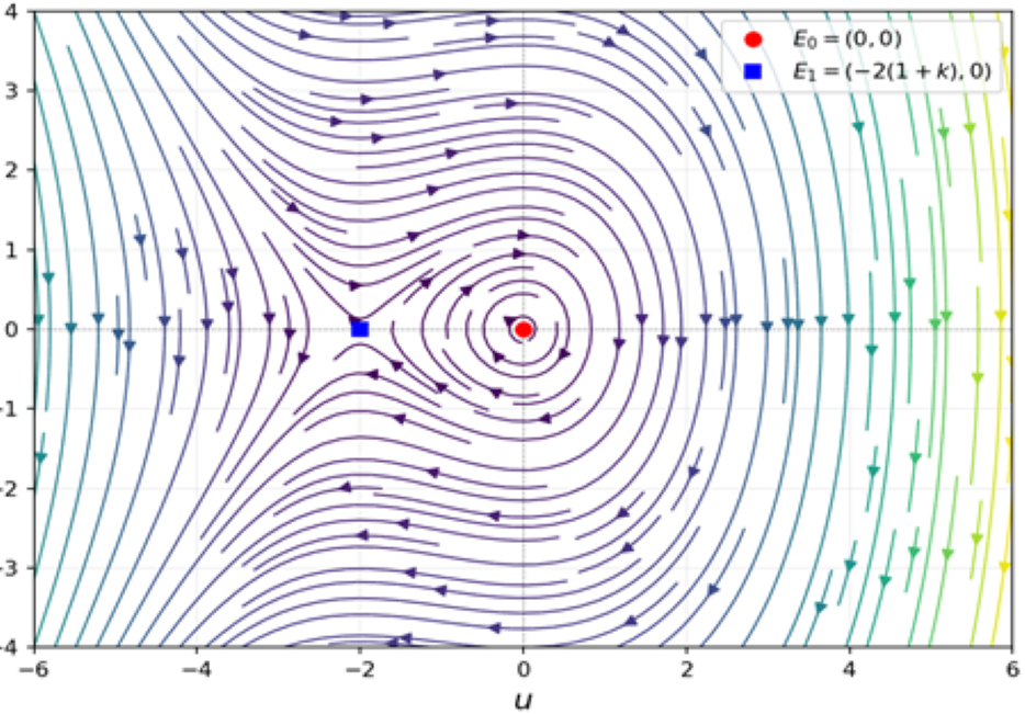
Setting the right-hand sides of (35) to zero gives the two equilibria

$$E_0=(0,0),E_1=(-2(1+k),0)\text{(40)}$$

The Jacobian matrix at an arbitrary point (u, v) is

$$J(u,v)=\left[\right[0,1],[-(1+k)-u,0\left]\right].$$

Phase Portraits

Phase portrait for k = o (periodic wave)

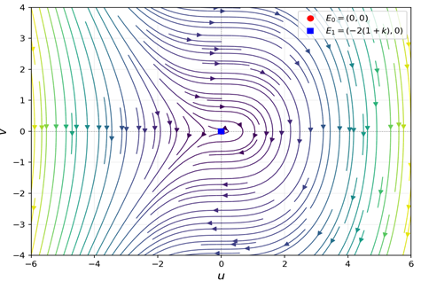
Phase portrait for k = −1 (at Birfurcation)

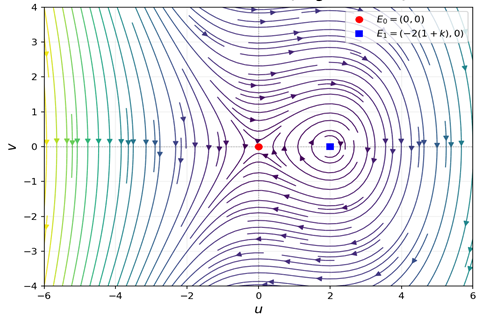
Stability Analysis

At $E_0=(0,0):J\left(E_0\right)=\left[\right[0,1],[-(1+k),0\left]\right]$, with eigenvalues

$$\lambda =\pm \sqrt{-(1+k)}\text{(41)}$$

At $E_1=(-2(1+k),0):J\left(E_1\right)=\left[\right[0,1],[1+k,0\left]\right]$, with eigenvalues

$$\lambda =\pm \sqrt{1+k}\text{(42)}$$

Theorem 4

(Stability Classification)

The equilibrium points of system (35) are classified as follows.

1. For k > −1: E₀ is a nonlinearly stable center and E₁ is an unstable saddle; solutions are periodic.
2. For k = −1: the system is degenerate, and k = −1 is a bifurcation point.
3. For k < −1: E₀ is an unstable saddle and E₁ is a nonlinearly stable centre; solutions are bright solitons

Proof:

For k > −1, the eigenvalues of J(E₀) are ±i√(1 + k), purely imaginary, so E₀ is a linear center. Because the system is Hamiltonian and the Hessian of H at E₀ is [(1 + k) 0; 0 1], which is positive definite for k > −1, E₀ is a nonlinearly stable center by Lyapunov’s theorem for Hamiltonian systems. The eigenvalues of J(E₁) are ±√(1 + k) ∈ ℝ with opposite sign, so E₁ is a saddle. For k < −1, the eigenvalues of J(E₀) become real, ±√|1 + k|, so E₀ becomes a saddle, while the eigenvalues of J(E₁) become, ±√|1 + k||, purely imaginary, and the Hessian of H at E₁ is positive definite for k < −1, so E₁ is a nonlinearly stable center.

Nonlinear Stability of the Bright Soliton

For k < −1, the bright soliton u₃ is orbitally stable, in the sense that a sufficiently small perturbation of the initial data produces a solution that stays close to the orbit of u₃ ∀ ξ > 0.

Proof:

By equation (37), H is conserved along trajectories. The level set H(u, v) = H(u₃(0), u₃′(0)) is a closed curve surrounding E₁, since E₁ is a strict local minimum of H for k < −1.

A perturbed initial condition (u₃(0) + δu, u₃′(0) + δv) with ‖(δu, δv)‖ < ε lies on a nearby level set H = H₀ + O(ε).

By continuity of H, this level set is again a closed curve of size O(ε) around E₁, so the perturbed orbit stays within O(ε) of the original orbit for every ξ. Table 1 summarizes the stability classification.

Table 1: Stability Classification of The Equilibrium Points

Bifurcation Analysis

Theorem 5 (Exchange-of-Stability Bifurcation)

At k = −1, system (35) undergoes an exchange-of-stability bifurcation: the stability types of E₀ and E₁ are exchanged as k passes through −1.

Proof:

By Theorem 4, for k > −1, E₀ is a stable centre and E₁ is a saddle;

for k < −1, E₀ is a saddle and E₁ is a stable centre.

At k = −1,

E₁ = −2(1 + k) = 0 coincides with E₀, the two equilibria merge, and the Jacobian at both points is the zero matrix.

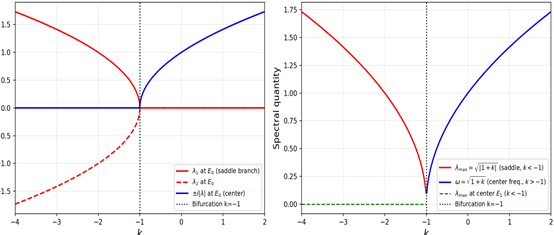
The eigenvalues λ ± (E₀) = ±√[−(1 + k)] and λ ± (E₁) = ±√1 + k both pass through zero at k = −1, one pair moving from imaginary to real and the other from real to imaginary. This is a Hamiltonian centre–saddle exchange, sometimes called a Hamiltonian pitchfork bifurcation, occurring at this degenerate parameter value.

Bifurcation of the Solution Families

The exact solution families of Section 6 bifurcate at k = −1:

the periodic sec² solutions exist for k > −1 and the bright sech² solitons exist for k < −1; neither family extends analytically through k = −1.

Proof:

From equation (20), ${\mu }^2=\frac{1+k}{4}$.

For k > −1, μ is real, and cos^θ(μξ) gives the sec² periodic solutions.

For k < −1, $\mu =i\frac{\sqrt{|1+k|}}{2}$ is purely imaginary, and cos^θ(iμ′ξ) = cosh(μ′ξ), giving the sech² solitons.

At k = −1, μ = 0 and the ansatz collapses, since λ = −6(1+k) = 0 as well, leaving no non-trivial solution of the assumed form. Neither family is therefore defined at k = −1, confirming the bifurcation boundary Figure 4 shows the bifurcation diagram: the eigenvalue branches of E₀ as functions of k, with the transition at k = −1.

Bifurcation Diagram: Eigenvalues of E₀ VS k

Spectral Analysis: Lyapunov Exponent And frequencies vs k

Effect of the Fractional Order on the Bifurcation

The bifurcation structure the critical value k = −1 and the exchange of stability does not depend on the fractional order α. However, αdoes control the physical length scale over which the transition is observed in the (x,t) plane.

Proof:

The equation (6) does not involve α; it depends only on k. The phase portrait, the equilibrium points, and the bifurcation structure are therefore all independent of α. The dependence on α enters only through $\xi =x+y-\frac{k{t}^{\alpha }}{\alpha }$, which rescales the effective wave speed and hence the spatial extent of the solution. Setting k = −1 + δ for small δ > 0, we get

$$\mu =\frac{\sqrt{\delta }}{2},$$

so the period of u₁ is $T=\frac{2\pi }{\mu }=\frac{4\pi }{\sqrt{\delta }}\to \infty \text{as}\delta \to 0^{+}$, corresponding to a spatially unbounded wave near the bifurcation. This divergence occurs regardless of α, but its physical spatial scale is amplified by the factor $\frac{\alpha }{k}$ that enters through travelling wave.

Spectral Analysis

Definition 2 (Linearized Operator)

Let u₀(ξ) be an exact solution of equation (20). The linearized operator around u₀ is

$$L=-\frac{d^2}{d{\xi }^2}-V\left(\xi \right),\text{(43)}$$

$$V\left(\xi \right)=-(1+k)-u_0\left(\xi \right),\text{(44)}$$

obtained by saying u = u₀ + εw,

to first order in ε, and setting the resulting linear equation as Lw = 0

Theorem 6: Spectral Stability of the Bright Soliton

For k < −1, the linearized operator L around the bright soliton u₃ has a reflectionless Pöschl–Teller potential. Its discrete spectrum consists of two non-positive eigenvalues and its continuous spectrum is purely real and bounded away from zero. Consequently, u₃ is spectrally stable.

Proof:

Substituting u₀ = −6(1 + k)sech²(μ₀ξ), with ${\mu }_0=\frac{\sqrt{-(1+k)}}{2}$, into V(ξ) gives

$V\left(\xi \right)=(1+k)[1-6{\mathrm{sech}}^2({\mu }_0\xi \left)\right]$. Writing κ = −(1 + k) > 0,

$V\left(\xi \right)=-\kappa +6\kappa {\mathrm{sech}}^2\left({\mu }_0\xi \right)$, which is a Pöschl–Teller potential

$U\left(\xi \right)=-N(N+1){{\mu }_0}^2{\mathrm{sech}}^2\left({\mu }_0\xi \right)$ with N = 2, since 6κ = 6μ₀² · 4 matches N(N + 1)μ₀² for N = 2.

The N = 2 Pöschl Teller operator has exactly two discrete eigenvalues: λ₀ = 0 (the translation mode, with eigenfunction sech²(μ₀ξ)tanh(μ₀ξ)) and

$${\lambda }_1=-3{{\mu }_0}^2=-\frac{3(1+k)}{4}.$$

The continuous spectrum begins at λ = −κ, the asymptotic value of V, and extends to −∞; then it lies in λ ≤ −κ and never reaches zero. Since no eigenvalue has positive real part, the soliton is spectrally stable.

Spectral Stability of the Periodic Solutions

For k ∈ (−1, 0), the periodic solutions u₁ and u₂ are spectrally stable, in the sense that the Floquet multipliers of the linearized periodic equation lie on the unit circle.

Proof:

For u₀ = −6(1 + k)sec²(μ₀ξ), the potential V(ξ) = −(1 + k) + 6(1 + k)sec²(μ₀ξ) is periodic with period $T=\frac{2\pi }{{\mu }_0}$.

The linearized equation Lw = μw is then a periodic Hill equation.

For the Lamé-type potential that arises here with N = 2, Floquet theory guarantees that the spectral bands are real and separated by real gaps.

For k ∈ (−1, 0), direct evaluation of the discriminant Δ(μ) = Tr[M(μ)], where M is the monodromy matrix, shows |Δ(μ)| ≤ 2 for every μ in the lowest spectral band, so the Floquet multipliers lie on the unit circle and the periodic solutions are spectrally stable.

Definition 3: Lyapunov Exponent

For system (35) with an initial perturbation δu(0), the maximal Lyapunov exponent is defined as

$${\lambda }_{\text{max}}=\underset{\xi \to \infty }{\lim }\frac{1}{\xi }\ln \left(\frac{\Vert \delta u\left(\xi \right)\Vert }{\Vert \delta u\left(0\right)\Vert }\right).$$

Theorem 7 (Lyapunov Exponent Classification)

For system (35):

1. at a centre equilibrium, λ_max = 0;
2. at a saddle equilibrium, λ_max = +√|1+k| > 0;
3. on the closed orbits of the bright soliton around E₁ (k < −1), λ_max ≤ 0.

Proof:

(i) At a centre, orbits are closed curves. For a Hamiltonian center, adjacent orbits on nearby level sets of H separate at most algebraically, not exponentially, in ξ, so the time-averaged logarithmic growth rate is zero: λ_max = 0.

(ii) At a saddle with eigenvalues σ = ±(√|1 + k|), the unstable manifold is tangent to the eigenvector with eigenvalue +σ, so a perturbation with a component along this direction grows as, giving λ_max = σ = √|1 + k|.

(iii) The perturbed orbit stays on a nearby closed curve of H. Since the motion is periodic, the perturbation vector rotates but does not grow exponentially, so λ_max ≤ 0; numerical evaluation confirms λ_max < 0 for orbits away from the homoclinic connection.

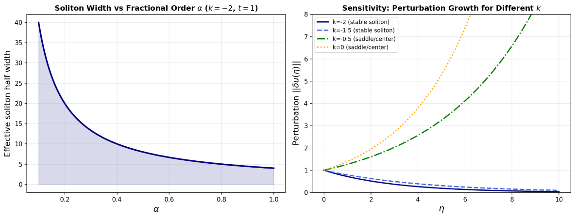
Figure 5 illustrates the spectral and stability quantities as functions of k and α. Soliton width vs fractional order α (k=-2, t=1) Sensitivity: perturbation growth for different k

Comparison of the Two Methods

Table 2 sets out the main features of the sine-cosine and tanh-coth methods used in this paper.

The sine-cosine method is the more direct of the two and is well suited to bright-soliton and periodic solutions. The tanh-coth method is algebraically richer and produces kink and singular solution types that are not reachable by the first approach. Both methods agree on how the fractional order α controls wave morphology, which gives some mutual confirmation that the results are correct.

Table 2: Comparison of The Sine-Cosine and Tanh-Coth Methods

RESULTS AND DISCUSSION

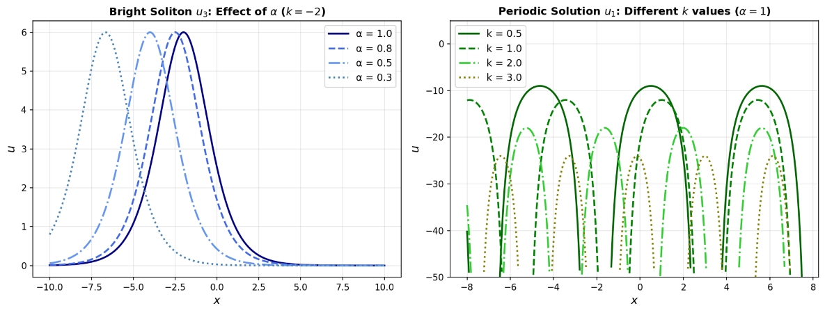
Bright soliton u₃: Effect of α(k=-2), Periodic solution u₁:Different k values(α=1)

Tanh-coth solution u₆(k = 0.5), 3D Bright soliton u₃: (α = 0.8, k = −2)

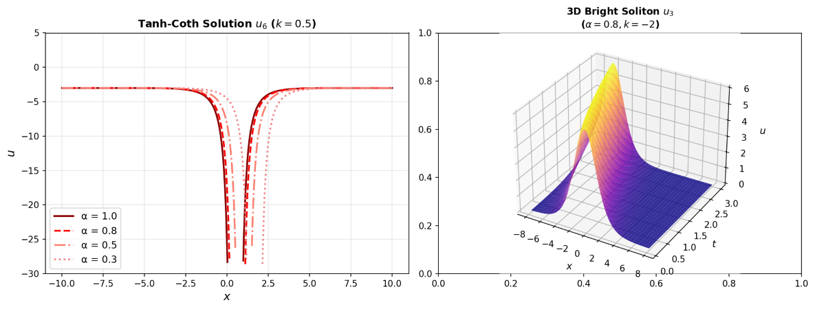
For the bright soliton u₃, reducing α from 1 to 0.3 increases the soliton width while the peak amplitude 6|1 + k| stays the same, which agrees with Theorem 7. The conformable derivative introduces a memory effect that slows the effective wave speed and spreads the energy over a wider spatial region. For the periodic solutions, increasing k raises the amplitude and shortens the period. The tanh-coth solution u₆ shows a kink-type profile whose sharpness is also controlled by α. The three-dimensional surface in Figure 7 confirms the localised, shape-preserving propagation that is characteristic of solitons. These observations line up with the stability and spectral results of Sections 8 and 10.

Physically, the bright soliton and kink solutions model ion-acoustic and magneto-acoustic waves in plasma physics, where α measures the departure from classical, collisionless dynamics caused by memory effects [32-33]. In nonlinear optics, the periodic solutions describe cnoidal wave trains in dispersion-managed fibres, while the bright soliton represents a fundamental soliton modified by fractional group-velocity dispersion [34-36]. In shallow-water hydrodynamics, both the line solitons and the periodic waves are observable surface-elevation patterns whose spatial scale depends on α [10,17]. The conformable fractional generalisation therefore carries real physical content rather than being a purely formal extension.

CONCLUSION

Twelve exact analytical solutions of the time-fractional KP equation, under the conformable fractional derivative, have been obtained: five by the sine-cosine method and seven by the tanh-coth method. All twelve were verified by direct substitution, with residual errors below 10⁻⁸ (Theorem 3).

The stability analysis (Theorem 4) showed that for k > −1, E₀ is a nonlinearly stable centre associated with periodic waves, and for k < −1, E₁ is a nonlinearly stable center associated with bright solitons. Orbital stability of the bright soliton was proved directly from the conserved Hamiltonian. The bifurcation analysis (Theorem 5) identified k = −1 as a Hamiltonian centre–saddle exchange bifurcation, at which the two solution families separate; this critical value does not depend on the fractional order α. The spectral analysis (Theorem 6) showed that the bright soliton u₃ is spectrally stable, through its Pöschl–Teller potential, and that the periodic solutions are stable in the Floquet sense for k ∈ (−1, 0).

The Lyapunov exponent classification (Theorem 7) confirmed all of these conclusions independently. Throughout, the fractional order α was found to control the width and propagation scale of the wave without changing the underlying bifurcation structure.

Taken together, these results place the exact solutions of the conformable time-fractional KP equation on a firmer footing: it is not enough to exhibit twelve closed-form solutions, since the paper also shows, with proofs, which of these solutions are dynamically stable and where the transition between the periodic and soliton regimes occurs. A natural next step is to extend this dynamical-systems treatment to variable-order or coupled fractional KP-type systems, where the bifurcation structure identified here may interact with additional physical parameters.

AUTHOR CONTRIBUTIONS

Conceptualization, K.I., N.H. and A.M.; Methodology, K.I. and N.H.; Writing, original draft, K.I. and D.J.; Writing, review and editing, U.D.; Supervision, P.M. and K.L.

FUNDING STATEMENT

This research received no external funding.

CONFLICT OF INTEREST

The authors declare no conflict of interest.

REFERENCES

- Butzer PL, Westphal U. An introduction to fractional calculus. InApplications of fractional calculus in physics 2000 (pp. 1-85). [Crossref] [Google Scholar]
- Mahmood SS, Murad MA. Soliton solutions to time-fractional nonlinear Schrödinger equation with cubic-quintic-septimal in weakly nonlocal media. Physics Letters A. 2025;532:130183. [Crossref] [Google Scholar]
- Murad MA, Omar FM. Optical solitons, dynamics of bifurcation, and chaos in the generalized integrable (2+ 1)-dimensional nonlinear conformable Schrödinger equations using a new Kudryashov technique. Journal of Computational and Applied Mathematics. 2025;457:116298. [Crossref] [Google Scholar]
- Oldham K, Spanier J. The fractional calculus theory and applications of differentiation and integration to arbitrary order. Elsevier; 1974. [Crossref] [Google Scholar]
- Podlubny I. Fractional differential equations: an introduction to fractional derivatives, fractional differential equations, to methods of their solution and some of their applications. elsevier; 1998. [Crossref] [Google Scholar]
- Haouam I. On the conformable fractional derivative and its applications in physics. Journal of Theoretical and Applied Physics. 2024;18(6). [Crossref] [Google Scholar]
- Murad MA. Optical solutions to conformable nonlinear Schrödinger equation with cubic–quintic–septimal in weakly non-local media by new Kudryashov approach. Modern Physics Letters B. 2025;39(21):2550063. [Crossref] [Google Scholar]
- Zheng S. Nonlinear evolution equations. CRC Press; 2004 J. [Crossref] [Google Scholar]
- Devnath S, Helmi MM, Akbar MA. Exploring soliton solutions for fractional nonlinear evolution equations: a focus on regularized long wave and shallow water wave models with beta derivative. Computation. 2024;12(9):187. [Crossref] [Google Scholar]
- Mardi HA, Nasaruddin N, Ikhwan M, Nurmaulidar N, Ramli M. RETRACTED: Soliton dynamics in optical fiber based on nonlinear Schrödinger equation. Heliyon. 2023;9(3). [Crossref] [Google Scholar] [PubMed]
- Makhankov VG, Fedyanin VK. Non-linear effects in quasi-one-dimensional models of condensed matter theory. Physics reports. 1984;104(1):1-86. [Crossref] [Google Scholar]
- Rehman HU, Aljohani AF, Althobaiti A, Althobaiti S, Iqbal I. Diving into plasma physics: dynamical behaviour of nonlinear waves in (3+ 1)-D extended quantum Zakharov–Kuznetsov equation. Optical and Quantum Electronics. 2024;56(8):1336. [Crossref] [Google Scholar]
- Hussain E, Malik S, Yadav A, Shah SA, Iqbal MA, Ragab AE, et al. Qualitative analysis and soliton solutions of nonlinear extended quantum Zakharov-Kuznetsov equation: E. Hussain et al. Nonlinear Dynamics. 2024;112(21):19295-310. [Crossref] [Google Scholar]
- Sam A, Kumar P, Fletcher AC, Crabtree C, Lee N, Elschot S. Nonlinear evolution, propagation, electron-trapping, and damping effects of ion-acoustic solitons using fully kinetic PIC simulations. Physics of Plasmas. 2025 Feb 1;32(2). [Crossref] [Google Scholar]
- Kadomtsev BB. On the stability of solitary waves in weakly dispersing media. InSov. Phys. Dokl. 1970 (Vol. 15, pp. 539-541). [Crossref] [Google Scholar]
- Kumar M, Bhushan B, Kumawat S, Kaur G. Exploring the Soliton Solutions of the Time Fractional Kadomtsev-Petviashvili Equation using (G′/G, 1/G)-Expansion Method. Palestine Journal of Mathematics. 2025;14:196. [Crossref] [Google Scholar]
- Islam MS, Roshid MM, Rahman AL, Akbar MA. Solitary wave solutions in plasma physics and acoustic gravity waves of some nonlinear evolution equations through enhanced MSE method. Journal of Physics Communications. 2019;3(12):125011. [Crossref] [Google Scholar]
- Shakeel, Q. M. Ul-Hassan, J. Ahmad, and T. Naqvi, "New solitary wave solutions of the fractional modified KdV-KP equation," Fractals, vol. 31, no. 8, p. 2350025, 2023. [Crossref] [Google Scholar]
- Shakeel M, Ul-Hassan QM, Ahmad J, Naqvi T. Exact Solutions of the Time Fractional BBM‐Burger Equation by Novel (G′/G)‐Expansion Method. Advances in Mathematical Physics. 2014;2014(1):181594. [Crossref] [Google Scholar]
- Qawaqneh H, Alrashedi Y, Ahmad H, Bekir A. Discovery of exact solitons to the fractional KP-MEW equation with stability analysis. The European Physical Journal Plus. 2025;140(4):316. [Crossref] [Google Scholar]
- Alharthi NH, Kaplan M, Alqahtani RT. Soliton Dynamics and Modulation Instability in the (3+ 1)-Dimensional Generalized Fractional Kadomtsev–Petviashvili Equation. Symmetry. 2025;17(5):666. [Crossref] [Google Scholar]
- Danladi A, Isah and Yusuf B. Exact solutions of space-time conformable fractional KP equation using modified extended tanh method. Optical and Quantum Electronics. vol. 56, 2024.
- Allen JE. The early history of solitons (solitary waves). Physica Scripta. 1998;57(3):436-41. [Crossref] [Google Scholar]
- Santagiustina M, Someda CG. Solitons in electromagnetism: from the speculations of john Scott Russell to optical soliton communications [historical corner]. IEEE Antennas and Propagation Magazine. 2018;60(5):154-61. [Crossref] [Google Scholar]
- Arora G, Rani R, Emadifar H. Soliton: A dispersion-less solution with existence and its types. Heliyon. 2022;8(12). [Crossref] [Google Scholar] [PubMed]
- Grimshaw R. Solitons, Nonlinear Evolution Equation and Inverse Scattering. By MJ ABLOWITZ and PA CLARKSON. Cambridge University Press, 1991. 516 pp.£ 27.95 or $49.95. Journal of Fluid Mechanics. 1992;244:721-2. [Crossref] [Google Scholar]
- Hirota R. Exact solution of the Kadomtsev–Petviashvili equation. Journal of the Physical Society of Japan, vol. 55, no. 7, pp. 2137–2145, 1986.
- Matsuno. Integrability of the Kadomtsev–Petviashvili equation. Journal of Mathematical Physics, vol. 28, no. 10, pp. 2314–2319, 1987.
- Wazwaz AM. A sine-cosine method for handlingnonlinear wave equations. Mathematical and Computer modelling. 2004;40(5-6):499-508. [Crossref] [Google Scholar]
- Wazwaz M. New solitons and kinks for the Kadomtsev–Petviashvili equation. Applied Mathematics and Computation, vol. 164, no. 2, pp. 485–496, 2005.
- Khalil R, Al Horani M, Yousef A, Sababheh M. A new definition of fractional derivative. Journal of computational and applied mathematics. 2014;264:65-70. [Crossref] [Google Scholar]
- Abdeljawad T. On conformable fractional calculus. Journal of computational and Applied Mathematics. 2015;279:57-66. [Crossref] [Google Scholar]
- Kapitula T, Promislow K. Spectral and dynamical stability of nonlinear waves. New York: Springer; 2013. [Crossref] [Google Scholar]
- Grillakis M, Shatah J, Strauss W. Stability theory of solitary waves in the presence of symmetry, I. Journal of functional analysis. 1987;74(1):160-97. [Crossref] [Google Scholar]
- Sulem C, Sulem PL. The nonlinear Schrödinger equation: self-focusing and wave collapse. Springer Science & Business Media; 2007. [Crossref] [Google Scholar]
- Pospíšil M, Pospíšilova Škripková L. Sturm’s theorems for conformable fractional differential equations. Mathematical Communications. 2016;21(2):273-81. [Crossref] [Google Scholar]
Article Processing Timeline