

 Download PDF
1Department of Mathematics, Mewar University, Chittorgarh, Rajasthan, India

Comparative Analysis of Correlation-Driven and Statistical Time Series Models for Financial Forecasting
Research Article - Volume: 1, Issue: 1, 2026 (September)
ABSTRACT
Financial time series forecasting is important for risk management, investment decision-making, and portfolio allocation. This study com- pares correlation-based analysis with classical statistical time-series modelling using daily NIFTY 50 data from January 2021 to December 2025. Pearson correlation analysis is used to examine contemporaneous relationships among key market variables, while logarithmic returns are analysed using stationarity tests, ACF/PACF analysis, and ARIMA modelling. Candidate ARIMA models are evaluated using AIC, AICc, BIC, and residual diagnostic tests. To assess predictive performance objectively, observations from 2021–2024 are used for model estimation, while 2025 is reserved for genuine out-of-sample one-step-ahead forecasting. The results show that correlation analysis provides useful information on market co-movement but does not itself constitute a forecasting model. The return series exhibits stationarity in the conditional mean, together with heavy tails and volatility-related dependence. ARIMA captures limited linear dependence in returns, but its forecasting performance remains constrained by un-modelled volatility dynamics. The findings support the use of ARIMA as an interpretable benchmark and highlight the potential value of volatility-aware and hybrid models for improved financial forecasting.
Keywords: Financial Time Series; NIFTY 50; Correlation Analysis; ARIMA; Forecasting; Stationarity; Volatility
INTRODUCTION
Forecasting financial markets is central to investors, portfolio managers, regulators, and policymakers, since accurate forecasts of price and return dynamics support risk management, capital allocation, and investment decision-making. Financial markets generate large volumes of sequential data characterized by uncertainty, volatility, and complex dependency structures, making reliable forecasting a persistent methodological challenge.
The NIFTY 50 index is the principal benchmark of the Indian equity market. As a value-weighted index of fifty large, representative companies listed on the National Stock Exchange of India (NSE), it provides a broad, sector-diversified indicator of aggregate market performance and is therefore a natural focus for empirical research on Indian financial time series [1,2].
Financial time series such as the NIFTY 50 typically display strong persistence in price levels, volatility clustering, heavy- tailed return distributions, and departures from normality [3,4], so naive forecasting approaches and models developed for stationary or Gaussian data are generally inadequate without appropriate transformation and diagnostic testing. Appropriate time series modelling therefore requires explicit treatment of stationarity, examination of the autocorrelation structure, and diagnostic assessment of model residuals. The autoregressive integrated moving average (ARIMA) framework provides a well-established, interpretable methodology for capturing linear dependence in the conditional mean of financial time series, commonly used together with unit-root and stationarity tests to establish the appropriate order of integration [4-6].
Correlation-based approaches offer a complementary perspective, focusing on contemporaneous linear association among financial variables such as price levels, trading volume, and return measures rather than the temporal dependence of a single series. Correlation analysis can reveal useful information about co-movement and market structure, but it does not, by itself, constitute a forecasting model. Motivated by this distinction, the present study undertakes an empirical comparison of correlation-based analysis and classical statistical time series modelling using daily NIFTY 50 data from January 2021 to December 2025. The statistical component is implemented through ARIMA, used to model the conditional mean of the return series; residual diagnostics further establish whether time-varying conditional variance remains, motivating volatility focused extensions such as ARCH/GARCH that are discussed as future work rather than estimated here. An extended five-year daily sample, with a strict chronological separation between a model-estimation period (2021–2024) and a genuine out-of-sample evaluation period (2025), allows the predictive value of the fitted model to be assessed under conditions that avoid look-ahead bias.
The primary objectives of this research are:
- To analyze correlation structures among financial time series variables.
- To apply classical time series analysis techniques for forecasting.
- To compare forecasting performance and interpretability of both approaches.
The empirical contribution lies in the joint application of descriptive, correlation, and ARIMA-based analysis to a validated, extended NIFTY 50 dataset, together with a genuine chronological out-of-sample forecasting evaluation that distinguishes predictability in the conditional mean from evidence of time-varying conditional variance.
The remainder of the paper proceeds as follows. Section Literature Review reviews the literature on financial time series forecasting, ARIMA modelling, volatility modelling, and recent NIFTY 50 evidence. Section: Data and Methodology describes the data and methodology, including data validation, descriptive statistics, correlation analysis, stationarity testing, ARIMA specification, and the out-of-sample forecasting design. Section Empirical Results and Discussion presents and discusses the empirical results. Section Conclusion concludes and outlines limitations and future research directions.
Literature Review
Forecasting financial time series has long combined classical statistical modelling with increasingly data-intensive methods, spanning traditional econometric methods, nonlinear statistical models, and, more recently, machine learning and deep-learning architectures [7]. Different forecast-accuracy measures possess different statistical properties and may lead to different conclusions about predictive performance; the Diebold–Mariano framework provides a formal statistical basis for testing whether differences in predictive accuracy are significant [8-9]. This methodological diversity motivates comparative empirical studies assessing the relative strengths of different forecasting frameworks under a common dataset.
The ARIMA framework remains foundational for univariate time series forecasting. Formalized by Box, Jenkins, Reinsel, and Ljung, it provides a systematic procedure for identifying, estimating, and diagnosing linear time series models through an iterative cycle of stationarity assessment, autocorrelation-based identification, and residual checking, with formal stationarity testing and residual diagnostics emphasized throughout the financial econometrics’ literature [5-6]. Recent work continues to benchmark ARIMA against alternative approaches; for instance, a comparative study of stock price prediction using artificial neural networks and ARIMA illustrates ARIMA’s continued relevance as a transparent statistical benchmark [10].
A closely related strand addresses time-varying conditional variance. The ARCH framework provides a formal basis for modelling such variance in financial returns: Engle’s original ARCH model showed that return-innovation variance can display predictable temporal structure, later generalized through the Generalized ARCH (GARCH) framework, and subsequent work established that volatility responds asymmetrically to positive and negative innovations [11-15]. Recent studies applying GARCH family models to Indian equity markets compare specifications for capturing NIFTY-level volatility and document asymmetric volatility effects and clustering in the NSE NIFTY 50, underscoring that conditional heteroskedasticity is a persistent, empirically important feature of Indian equity index returns distinct from linear dependence in the conditional mean [16-17].
Empirical research on the NIFTY 50 continues to develop, including analysis of its technical and time-series market-cycle characteristics and evidence of conditional heteroskedasticity and volatility persistence [18-23]. More recent studies investigate ARIMA, GARCH, and hybrid forecasting approaches for the NIFTY 50 and its constituent securities [10,16,17,18,24]. This literature, together with regulatory and index level documentation from SEBI and NSE Indices Limited, provides institutional and empirical context for the present study [1,2].
Beyond classical linear and volatility models, recent research increasingly explores hybrid and machine-learning-based forecasting: nonlinear time series and deep-learning approaches applied to an emerging financial market, and frameworks systematically comparing econometric, machine learning, and deep-learning models [7,25]. These contributions combine the interpretability of classical econometric models with the flexibility of data driven methods, particularly for capturing nonlinear and volatility-related structure that purely linear models may not represent.
Taken together, classical ARIMA modelling remains a useful, interpretable benchmark for the conditional mean of financial returns; conditional heteroskedasticity is a well-documented feature of Indian equity index returns; and hybrid/machine-learning approaches are increasingly applied alongside these traditional tools. Relatively fewer studies jointly examine correlation based descriptive analysis and formally validated ARIMA modelling on an extended, systematically cleaned NIFTY 50 dataset with a genuine chronological out-of-sample evaluation. The present study addresses this gap by combining correlation analysis, rigorous stationarity testing, ARIMA identification and diagnostic checking, and out-of-sample forecast evaluation within a single, internally consistent framework applied to five years of daily NIFTY 50 data.
DATA AND METHODOLOGY
Data Description and PreprocessingThe empirical investigation employs daily observations of the NIFTY 50 index from January 2021 through December 2025, sourced from the Investing.com financial data portal, containing date, opening price, intraday high, intraday low, closing price, trading volume, and daily percentage change [26]. The NIFTY 50 is the principal benchmark equity index of the NSE, comprising 50 large, representative companies, making it an appropriate market-level indicator for examining the statistical behaviour and short-term predictability of Indian equity prices.
The five-year daily window provides a substantially larger empirical basis for statistical inference than shorter windows used in related studies, incorporating observations from different market conditions and thus greater variation for examining price co-movement, return dynamics, and forecasting performance.
The empirical analysis has two chronological components: observations from 2021–2024 (the training sample) are used for exploratory analysis, model identification, parameter estimation, and diagnostic testing, while 2025 observations form a strictly out-of-sample testing period not used during estimation. Forecasts from the models estimated on the training sample are subsequently compared with observed 2025 values, reducing look-ahead bias and providing a more realistic assessment of predictive performance.
Price levels are used for descriptive properties and contemporaneous relationships among market variables, whereas logarithmic returns serve as the principal series for stationarity, autocorrelation, ARIMA, and forecasting analysis. Trading volume is incorporated into the correlation analysis to examine whether changes in market participation are associated with NIFTY 50 movements.
Before the statistical analyses, the raw NIFTY 50 dataset was subjected to a systematic validation and cleaning procedure to ensure internally consistent observations and prevent data-quality issues from biasing subsequent inference. All dates were converted to a uniform format and arranged chronologically, and the dataset was examined for duplicate dates, invalid entries, missing prices, and non-positive values. Internal consistency of the daily open–high–low–close (OHLC) variables was verified using
(1)
(2)
where O t , H t , L t , and C t denote the opening, high, low, and closing prices at observation t , ensuring the reported daily high is never below the opening or closing price and the reported daily low never above them. The trading-volume variable was evaluated separately because volume information was unavailable for two observations (20 January 2024 and 19 February 2024). Since the corresponding price observations were available and internally consistent, these observations were retained in the master price and return dataset; no artificial values were generated through interpolation, extrapolation, or imputation. The unavailable volume observations were treated as missing and excluded only from analyses explicitly requiring volume information, so that the complete validated price series is used for constructing logarithmic returns and subsequent time-series modelling, while volume-dependent statistics use only observations where volume is available. The dataset was also checked for dates outside the regular Monday–Friday trading calendar; such dates were evaluated individually rather than automatically removed, since the Indian equity market occasionally conducts officially scheduled special sessions. The resulting validated dataset, summarized in Table 1, was designated the master dataset, with no further observation-level modifications made before analysis.
Descriptive Statistics
Descriptive statistics were computed for the opening, high, low, and closing prices, trading volume, and logarithmic returns: the number of observations ( N ), mean, median, standard deviation, minimum, maximum, skewness, and excess kurtosis.
The mean of a variable X is
(3)
with the median, a robust measure particularly useful under asymme-try, reported alongside it. Dispersion is measured by the sample standard deviation,
| Validation criterion | Result | Treatment | Status |
|---|---|---|---|
| Total observations | 1,240 | Complete daily dataset retained for the empirical analysis | Retained |
| Invalid dates | 0 | No invalid or unparseable dates identified | Passed |
| Duplicate dates | 0 | No duplicate date observations identified | Passed |
| Missing price values | 0 | No missing observations in the price variables | Passed |
| Non-positive prices | 0 | No zero or negative price observations identified | Passed |
| OHLC inconsistencies | 0 | All observations satisfy the specified high/low consistency conditions | Passed |
| Missing volume | 2 | Volume unavailable for 20-Jan-2024 and 19-Feb-2024; no imputation performed | Controlled |
| Special trading dates | Reviewed | Non-standard trading dates were individually evaluated rather than automatically deleted | Retained |
| Chronological ordering | Valid | Observations arranged chronologically before time-series analysis | Passed |
| Final master dataset | 1,240 | Validated dataset used for subsequent empirical analysis | Final |
Table 1: Data Validation and Cleaning Procedure for the NIFTY 50 Dataset
(4)
and the observed range,
(5)
Distributional symmetry is assessed via skewness,
where positive (negative) values indicate upper(lower-) tail asymmetry,and tail behaviour via excess kurtosis,
where the subtraction of three sets the normal distribution benchmarkto zero; positive values indicate heavier tails and a greater propensity forextreme observations.
Particular attention is given to logarithmic returns, computed from consecutive closing prices as
(8)
examined separately from the price-level variables and, in addition to the full sample, separately for the training period (2021–2024) and the out-of-sample period(2025) to assess whether distributional characteristics changed between the two.
Pearson Correlation Analysis
The Pearson product–moment correlation coefficient was computed for the opening, high, low, and closing prices, trading volume, and percentage price change, to assess the extent to which movements in one market variable are linearly associated with another. For variables X and Y,
with and the respective sample means and
A positive (negative) coefficient indicates co-movement in the same (opposite) direction, and magnitude reflects linear strength rather than causality.
The correlation matrix uses pairwise complete observations: price–price correlations use the full price sample, while correlations involving volume use only observations where volume is available, with no imputation. Strong contemporaneous association among the open, high, low, and close prices is expected because these are generated within the same trading day and reflects co-movement and intraday price structure rather than an indepen-dent predictive relationship. The correlation between volume and percentage price change is examined separately, and results are subsequently considered alongside the time- series analysis to determine whether contemporaneous as-sociation is accompanied by serial dependence useful for forecasting.
Return Construction and Stationarity Testing
The NIFTY 50 closing-price series was transformed into continuously compounded logarithmic returns,
(11)
with Pt the closing price at time t, producing 1,239 valid return observa-tions from 1,240 daily prices (the first observation lacks a preceding closing price).
Rather than assuming stationarity follows automatically from the log transformation, the resulting series was formally evaluated using two complementary tests with opposite null hypotheses: the Augmented Dickey–Fuller (ADF) test [27] and the Kwiatkowski–Phillips–Schmidt–Shin (KPSS) test [28].
Augmented Dickey–Fuller Test
The ADF test examines the null hypothesis of a unit root [27] via the augmented regression
(12)
where ∆ is the first-difference operator, α an intercept, β t an optional deterministic trend, γ the unit-root test coefficient, p the number of lagged difference terms, and ε t an innovation, with hypotheses
(13)
and
(14)
Lag length is selected via the Akaike Information Criterion to reduce residual serial correlation while avoiding unnecessary parameterization; the decision rule is based on the reported probability value against critical values.
Kwiatkowski–Phillips–Schmidt–Shin Test
The KPSS test [28] takes stationarity as its null hypothesis, in contrast to ADF:
(15)
against
(16)
The statistic is constructed from the partial sums of residuals after removing the deterministic component,
(17)
where,
(18)
is the cumulative residual sum and σ b 2 a consistent long-run variance es-timate. For price levels the assessment allows a deterministic trend, while returns are assessed around a constant mean.
Stationarity is considered strongly supported when ADF rejects the unit-root null while KPSS fails to reject its stationarity null; this combined evi-dence, together with ACF/PACF analysis, determines whether an integrated component is required for the forecasting model.
Autocorrelation and Partial Autocorrelation Analysis
The temporal dependence structure of the return series was examined using the sample autocorrelation function (ACF) and partial autocorrelation function (PACF), providing an empirical basis for specifying the AR and MA orders of the ARIMA model [5]. For a stationary series {r t }, the sample autocorrelation at lag k is
where r¯ is the sample mean return; the PACF measures the correlation between r t and r t−k after removing the linear e˙ects of intermediate lags r t−1 , . . . , r t−k+1 , distinguishing direct lag dependence from dependence transmitted through shorter lags. For sufficiently large samples, approximate 95%confidence limits are
(20)
with spikes outside these limits providing preliminary evidence of serial dependence, interpreted jointly with information criteria and residual diagnostics rather than as the sole model- selection criterion.
A rapid ACF decay with a dominant first-lag PACF spike would support a low-order autoregressive component; a sharp ACF cutoff with gradually declining PACF would suggest a moving-average structure; gradual decay in both may indicate a mixed ARMA specification. These patterns are used to construct a small set of candidate ARIMA models, subsequently compared using the Akaike (AIC) and Bayesian (BIC) information criteria and residualdiagnostics, ensuring model identification is supported by both the observed dependence structure and formal diagnostics.
ARIMA Model Specification
The ARIMA framework was employed to model and forecast the conditional mean of the NIFTY 50 return series, providing a systematic representation of temporal dependence through autoregressive and moving- average compo-nents while allowing for non-stationarity through differencing [5-6], used here as an interpretable benchmark for assessing how much historical return information contributes to short-term forecasting performance.
The general ARIMA(p, d, q) model is
where B is the backshift operator, d the differencing order, p the AR order, q the MA order, c a constant, and an innovation, with polynomials
and
The AR component captures dependence on previous returns, the MA component dependence on previous innovations/forecast errors, and the integration component accommodates non-stationarity through differencing [4-5].
Determination of the Integration Order
The integration order was determined from the stationarity analysis in Sec-tion 3.4, using ADF (unit- root null) and KPSS (stationarity null) as comple-mentary tests [27-28]. Since the combined evidence supported stationarity of the return series, no further differencing was applied:
(24)
reducing the ARIMA framework to an ARMA specification for the return process,
(25)
consistent with the standard finding that financial returns are typically more stationary than the corresponding price levels [4,6]. Stationarity of the conditional mean does not, however, imply constant conditional variance; the residual diagnostics in Section 3.7 separately examine whether volatility-related dependence remains after fitting.
Identification of the AR and MA Orders
The AR order p and MA order q were investigated using the ACF/PACF (Section 3.5), which in the classical Box–Jenkins framework provide initial information for identifying plausible structures [5]. Because financial return series often exhibit weak, rapidly declining autocorrelation, a final model was not selected from visual inspection alone; instead, the ACF/PACF analysis defined a parsimonious candidate set, subsequently compared using formal information criteria and residual diagnostics. The following low-order candidates were considered:
(26)
This low-order set provides sufficient flexibility to capture short-term lin-ear dependence while avoiding unnecessary parameterization; ARIMA(0, 0, 0) is included as a particularly important benchmark, corresponding to a con-stant conditional-mean specification with no serial dependence beyond the estimated mean.
Model Estimation and Selection
All candidates were estimated on the 2021–2024 training sample (990 return observations); the 2025 observations were reserved exclusively for the subsequent out-of- sample evaluation, ensuring this information could not in-fluence the estimated model. Candidates were compared using the Akaike Information Criterion (AIC), corrected AIC (AICc), and Bayesian Informa-tion Criterion (BIC) [4-5]:
(27)
(28)
(29)
where ℓ is the maximized log-likelihood, k the number of estimated parameters, and N the effective sample size; lower values indicate a preferred model. These criteria were not the sole basis for selection: a candidate was preferred only when its information-criterion performance was supported by statistically adequate residual behaviour, following the Box–Jenkins principle that identification should be followed by estimation and diagnostic checking rather than an automated numerical rule alone [5].
Interpretation of the ARIMA Model in the Financial Context
The ARIMA framework here captures linear dependence in the conditional mean; financial returns may show limited such dependence while exhibiting substantial dependence in conditional variance [4,11,12]. An ARIMA model with approximately uncorrelated residuals should not therefore be read as ev-idence that the return process is completely unpredictable, but that its linear conditional-mean information has been substantially accounted for; remain-ing dependence in squared or absolute residuals may indicate predictable volatility dynamics requiring a separate conditional-variance model such as ARCH or GARCH [11,12]. Given the substantial excess kurtosis and clus-tered large returns evident in the descriptive analysis, the ARIMA model is evaluated primarily as a conditional-mean forecasting model, with remaining volatility structure investigated via the ARCH-LM diagnostic (Section 3.7). The selected specification is finally used to generate one-step-ahead forecasts for 2025, evaluated using MAE, RMSE, MFE, and directional accuracy (Section 3.8), permitting a clear distinction between in-sample adequacy and genuine out-of-sample performance.
Model Estimation and Diagnostic Checking
Model comparison used AIC, AICc, and BIC [29,30], as defined in Equa-tions (27-29) above, balanced against parameter significance and residual diagnostics rather than used in isolation. The Ljung–Box test [31] was ap-plied to model residuals to check for remaining serial correlation, the Jarque–Bera test [32] to evaluate residual normality, and the ARCH-LM test, based on the ARCH framework [11], to assess residual conditional heteroskedastic-ity. Together, these diagnostics distinguish adequacy of the conditional-mean specification from remaining distributional or volatility-related residual structure, providing a data-driven basis for model selection rather than relying on an assumed or arbitrarily preferred specification. Following the candidate- model comparison, the selected specification was re-estimated using a numerically stabilized maximum-likelihood procedure to ensure convergence; the return series was rescaled during optimization, with resulting parameter estimates and forecasts transformed back to the original return scale.
Forecasting Methodology
A genuine out-of-sample forecasting experiment evaluated the selected ARIMA model’s practical performance: for each 2025 trading day, a one-step-ahead forecast used only information available up to the preceding observation, compared with the corresponding realized return. The forecast error for observation t is
(30)
with accuracy evaluated via mean absolute error (MAE) and root mean squared error (RMSE),.
(32)
and mean forecast error (MFE), assessing bias:
(33)
Because percentage-based measures such as MAPE can be unstable for returns near zero or changing sign, directional accuracy is reported instead as an additional practical measure,
(34)
where I [ · ] is an indicator function.
Out-of-Sample Forecasting and Model Evaluation
Following the chronological design in Section 3.1, the 990 daily return observations from 2021–2024 were used exclusively for estimation, while the 249 observations from 2025 were retained as an unseen evaluation sample.
EMPERICAL RESULTS AND DISCUSSION
This section presents the empirical findings from the cleaned 2021–2025 NIFTY 50 dataset, proceeding from descriptive statistics of market variables to return behaviour, formal stationarity testing, conditional-mean identification, residual diagnostics, and out-of-sample forecasting, emphasizing throughout the distinction between predictability in the conditional mean and persistence in the conditional variance.
Descriptive Characteristics of the NIFTY 50 Series
Figure 1 shows the NIFTY 50 closing price over 2021–2025: a clear long-run upward movement, interrupted by substantial short-term corrections, rising from approximately 14,000 at the start of 2021 to above 26,000 by late 2025. The intermediate declines and recoveries indicate a strongly persistent but non-monotonic price level, an initial indication of non-stationarity motivating the transformation to logarithmic returns.
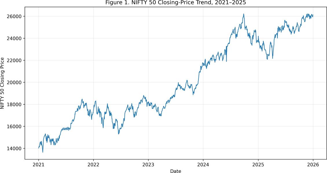
Figure 1:NIFTY 50 closing-price trend, 2021–2025.
Table 2 reports descriptive statistics of the market variables. The price variables are broadly similar: mean opening price 20,062.2405 versus mean closing price 20,053.9756, with standard deviations 3,581.1286 and 3,583.0412, respectively, reflecting common underlying price dynamics. The closing price ranges from 13,634.60 to 26,216.05 (mean 20,053.9756, median 19,063.4250, mean > median), with positive skewness (0.2085) indicating modest rightward asymmetry; the open, high, and low variables show similar skewness (0.2071–0.2113) and negative excess kurtosis (−1.3503 to −1.3658), indicat-ing flatter-than-Gaussian price-level distributions.
Trading volume behaves quite differently: mean 318.7135 million versus median 283.2000 million (SD 125.7744 million; range 19.06–1,100.00 million), with skewness 1.9418 and excess kurtosis 5.5832, indicating pronounced positive asymmetry and heavy tails consistent with occasional exceptionally high- volume days. The volume variable contains 1,236 observations versus 1,240 for prices, the two unavailable observations retained as missing rather than imputed (Section 3.1).
| Variable | N | Mean | Median | SD | Minimum | Maximum | Skewness | Excess Kurtosis |
|---|---|---|---|---|---|---|---|---|
| Open | 1240 | 20062.2405 | 19058.7250 | 3581.1286 | 13758.60 | 26325.80 | 0.2087 | -1.3592 |
| High | 1240 | 20150.6923 | 19127.2750 | 3590.0714 | 13898.25 | 26325.80 | 0.2113 | -1.3658 |
| Low | 1240 | 19950.9863 | 18956.8500 | 3579.2835 | 13596.75 | 26172.40 | 0.2071 | -1.3503 |
| Close | 1240 | 20053.9756 | 19063.4250 | 3583.0412 | 13634.60 | 26216.05 | 0.2085 | -1.3581 |
Table 2: Descriptive statistics of NIFTY 50 market variables, 2021–2025
Figure 2 shows the resulting daily logarithmic-return series, fluctuating around zero with small movements on most days but occasional large positive and negative innovations; the clustering of periods with larger absolute returns provides preliminary visual evidence of time-varying volatility.
Table 3 reports return statistics for 2021–2024, 2025, and the full sample (1,239 observations, one fewer than closing prices as expected). For 2021–2024, mean 0.000528, median 0.000823, SD 0.009124 (substantially larger than the mean), range −0.061124 to 0.046333, skewness −0.530077 (moderate negative asymmetry), excess kurtosis 4.334275 (heavy tails). The 2025 sample shows lower dispersion (SD 0.007429; mean 0.000401, median 0.000012, range −0.032970 to 0.037472) but with skewness reversing sign to positive (0.276397) while excess kurtosis remains substantial (3.583739), so heavy-tailed behaviour persists despite the change in asymmetry direction. For the full sample, mean 0.000503, median 0.000550, SD 0.008807, range−0.061124 to 0.046333, skewness −0.435115, excess kurtosis 4.394124. Figure 3 further illustrates the distribution: a histogram concentrated around zero with visibly extended tails relative to the superimposed normal reference density, consistent with the positive excess kurtosis in Table 3 and the negative full-sample skewness.
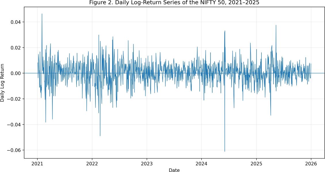
Figure 2:Daily logarithmic returns of the NIFTY 50, 2021–2025.
| Sample | N | Mean | Median | SD | Minimum | Maximum | Skewness | Excess Kurtosis |
|---|---|---|---|---|---|---|---|---|
| 2021–2024 | 990 | 0.000528 | 0.000823 | 0.009124 | -0.061124 | 0.046333 | -0.530077 | 4.334275 |
| 2025 | 249 | 0.000401 | 0.000012 | 0.007429 | -0.032970 | 0.037472 | 0.276397 | 3.583739 |
| Full sample | 1239 | 0.000503 | 0.000550 | 0.008807 | -0.061124 | 0.046333 | -0.435115 | 4.394124 |
Table 3: Descriptive statistics of NIFTY 50 logarithmic returns
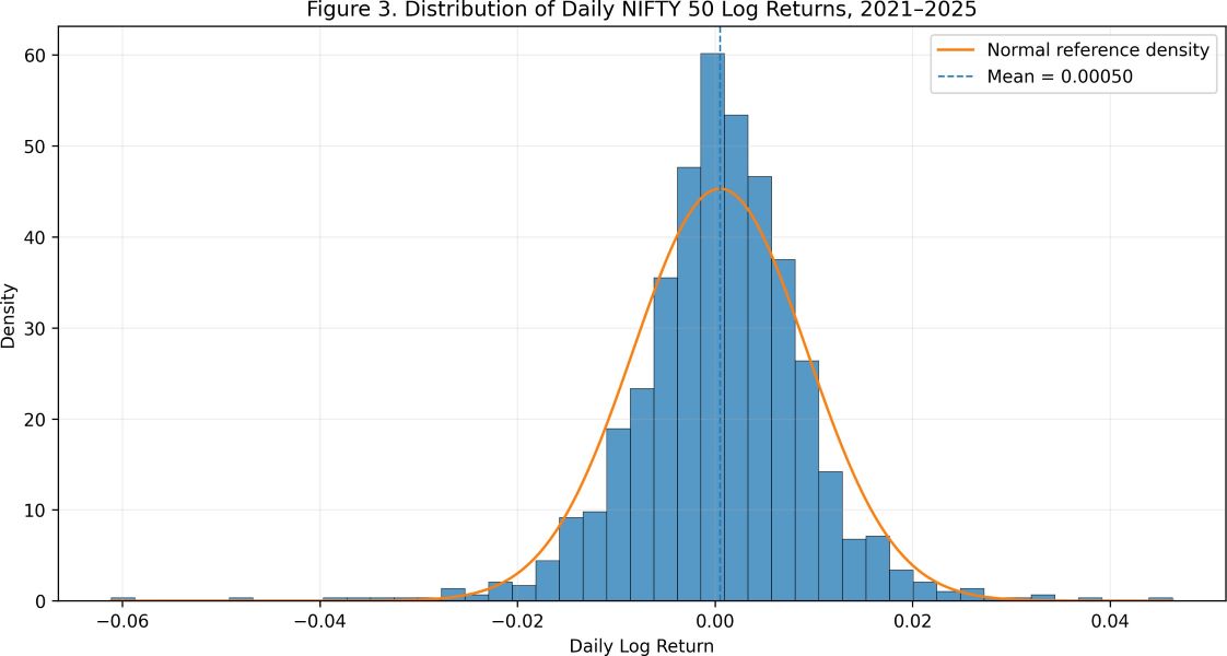
Figure 3:Distribution of daily NIFTY 50 logarithmic returns, 2021–2025, with a normal reference density.
Overall, the descriptive evidence establishes three features of the NIFTY 50 return process: the mean daily return is small relative to its standard deviation, indicating substantial short-term uncertainty around the condi-tional mean; the return distribution is asymmetric, with the direction of skewness differing between the estimation and evaluation periods; and positive excess kurtosis in both periods demonstrates persistent departure from normality. These characteristics motivate the subsequent stationarity tests, conditional-mean modelling, residual diagnostics, and explicit consideration of conditional variance dynamics.
Correlation Results
Table 4 reports the Pearson correlation matrix. Price-related variables are strongly associated (open/high/low/ close pairwise correlations all exceeding 0.999), expected since these represent the same daily trading process.
Trading volume shows a moderate negative correlation with price levels (−0.216703 to −0.228086) and a weak negative correlation with percent-age price change (−0.035694); percentage price change itself correlates only weakly with price levels (−0.017910 to 0.012302).
The strong price-level associations should not be read as evidence of return predictability: price levels are highly persistent and can display substantial contemporaneous correlation even when successive returns show little linear dependence, and volume’s contemporaneous association with price movements does not by itself establish predictive causality. The correlation analysis is therefore a descriptive diagnostic rather than evidence of a forecasting relationship, supporting the decision to avoid modelling persistent price levels directly and instead focus the forecasting analysis on logarithmic returns, for which stationarity and serial dependence can be assessed more appropriately.
| Open | High | Low | Close | Volume | Change (%) | |
|---|---|---|---|---|---|---|
| Open | 1.000000 | 0.999731 | 0.999557 | 0.999247 | -0.220580 | -0.017910 |
| High | 0.999731 | 1.000000 | 0.999538 | 0.999656 | -0.216703 | -0.006017 |
| Low | 0.999557 | 0.999538 | 1.000000 | 0.999693 | -0.228086 | -0.000216 |
| Close | 0.999247 | 0.999656 | 0.999693 | 1.000000 | -0.222466 | 0.012302 |
| Volume | -0.220580 | -0.216703 | -0.228086 | -0.222466 | 1.000000 | -0.035694 |
| Change (%) | -0.017910 | -0.006017 | -0.000216 | 0.012302 | -0.035694 | 1.000000 |
Table 4:Pearson correlation matrix of NIFTY 50 market variables, 2021–2025
Stationarity Results
Table 5 reports ADF and KPSS results, showing fundamentally different stochastic properties for prices versus returns.
| Series | ADF Statistic | ADF p-value | KPSS Statistic | KPSS p-value | Conclusion |
|---|---|---|---|---|---|
| Close Price | -2.7913 | 0.2001 | 0.487 | 0.01 | Non-stationary |
| Log Returns | -34.7372 | < 0.001 | 0.0391 | > 0.100 | Stationary |
Table 5: ADF And KPSS Stationarity Tests for The NIFTY 50 Series
For closing prices, the ADF statistic ( − 2.7913, p = 0.2001) fails to reject the unit-root null, while KPSS (0.4870, p ≈ 0.01) rejects level stationarity, so the price series is treated as non-stationary. For the full-sample log returns, ADF ( − 34.7372, p < 0.001) rejects the unit-root null and KPSS (0.0391, p > 0.10) fails to reject stationarity, providing consistent evidence of return stationarity. The same conclusion holds separately for 2021–2024 (ADF − 15.8559, p < 0.001; KPSS 0.0461, p > 0.10) and 2025 (ADF − 15.3987, p < 0.001; KPSS 0.0511, p > 0.10), strengthening the justification for modelling returns without further differencing.
Accordingly, the ARIMA integration order is set to d = 0: the return process’s mean and autocovariance structure can be analysed without differencing, though this stationarity finding is distinct from predictability it does not imply future returns can be predicted accurately from past values. Remaining temporal dependence is examined next via ACF/PACF.
ARIMA Estimation Results
Figure 6 presents the sample ACF and PACF; both show limited significant structure across examined lags, preliminary evidence that persistent linear dependence in the conditional mean of daily returns is weak.
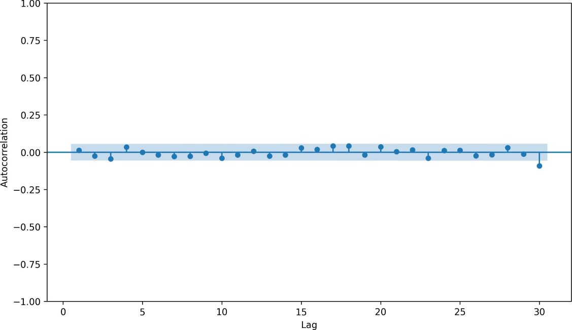
Figure 4:(a) *ACF
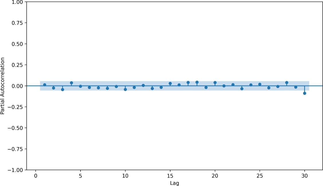
Figure 6 : Autocorrelation and partial autocorrelation functions of NIFTY 50 logarithmic returns, 2021–2025
Table 6 reports AIC, AICc, BIC, and Ljung–Box p-values (lag 20) for the nine candidates. ARIMA (0, 0, 0) yields the lowest values on all three information criteria (AIC = − 6487.333, AICc = − 6487.321, BIC = − 6477.538); ARIMA (1, 0, 0) and ARIMA (0, 0, 1) are only marginally higher, not enough to justify additional dynamic parameters.
The estimated ARIMA (1, 0, 0) AR coefficient ( φ ˆ 1 = 0.0112, p = 0.589) and ARIMA (0, 0, 1) MA coefficient (ˆ θ 1 = 0.0093, p = 0.652) are both statistically insignificant, consistent with the weak ACF/PACF structure in Figure 6. Ljung–Box tests do not reject the no-residual-autocorrelation null for the candidates; for ARIMA (0, 0, 0), p ≈ 0.455 at lag 10 and 0.744 at lag 20.
Accordingly, the candidate-model comparison does not support selecting ARIMA (1, 0, 0) over the constant- mean alternative. The evidence instead favours the more parsimonious ARIMA (0, 0, 0) representation,
(35)
| Model | AIC | AICc | BIC | LB p-value (20) |
|---|---|---|---|---|
| ARIMA (0, 0, 0) | -6487.333 | -6487.321 | -6477.538 | 0.744 |
| ARIMA (0, 0, 1) | -6485.461 | -6485.436 | -6470.767 | 0.757 |
| ARIMA (1, 0, 0) | -6485.458 | -6485.434 | -6470.765 | 0.758 |
| ARIMA (2, 0, 0) | -6484.619 | -6484.579 | -6465.028 | 0.819 |
| ARIMA (0, 0, 2) | -6484.443 | -6484.402 | -6464.852 | 0.811 |
| ARIMA (1, 0, 1) | -6483.334 | -6483.294 | -6463.743 | 0.744 |
| ARIMA (2, 0, 1) | -6481.334 | -6481.273 | -6456.846 | 0.744 |
| ARIMA (1, 0, 2) | -6482.182 | -6482.121 | -6457.693 | 0.798 |
| ARIMA (2, 0, 2) | -6482.799 | -6482.713 | -6453.413 | 0.925 |
Table 6: Comparison of candidate ARIMA models using information criteria and Ljung–Box diagnostics
The selected ARIMA (0, 0, 0) specification was re-estimated using a numerically stabilized maximum-likelihood procedure after an initial convergence warning; the stabilized estimation converged successfully, giving
(36)
(37)
(innovation SD ≈ 0.00912). Original-scale information criteria remain AIC = − 6487.333 and BIC = − 6477.538, so numerical stabilization does not alter the model-selection result, and successful convergence provides a further quality- control check for the subsequent diagnostics and forecasts.
Diagnostic Results
Table 7 reports residual diagnostics for the ARIMA (0, 0, 0) model. Ljung– Box shows no significant remaining serial correlation (Q (10) = 9.8374, p = 0.4549; Q (20) = 15.5451, p = 0.7444), supporting adequacy of the linear conditional- mean fit.
In contrast, the Jarque–Bera test decisively rejects residual normality (JB = 811.1924, p = 7.11 × 10 − 177), with negative skewness ( − 0.5301) and excess kurtosis (4.3343) indicating a negatively asymmetric, heavy-tailed distribution – so while the conditional mean is adequately captured, the Gaussian residual assumption is inappropriate [32]. The ARCH-LM test strongly rejects the no-ARCH- effects null across lags 5, 10, and 20 (statistics 81.9845, 92.0462, 106.9755; p = 3.22 ×10⁻¹⁶, 2.10 × 10⁻¹⁵, 6.97 × 10⁻¹⁴, respectively), providing strong evidence of conditional heteroskedasticity [11].
| Test | Lag | Statistic | p-value | Decision |
|---|---|---|---|---|
| Ljung–Box | 10 | 9.8374 | 0.4549 | Do not reject H0 |
| Ljung–Box | 20 | 15.5451 | 0.7444 | Do not reject H0 |
| Jarque–Bera | – | 811.1924 | 7.11 × 10−177 | Reject H0 |
| ARCH-LM | 5 | 81.9845 | 3.22 × 10⁻¹⁶ | Reject H0 |
| ARCH-LM | 10 | 92.0462 | 2.10 × 10⁻¹⁵ | Reject H0 |
| ARCH-LM | 20 | 106.9755 | 6.97 × 10⁻¹⁴ | Reject H0 |
Table 7: Residual diagnostic results for the ARIMA(0, 0, 0) model
Out-of-Sample Forecasting Results
The final forecasting evaluation, following Section Out-of-Sample Forecasting and Model Evaluation, used the 990 2021– 2024 observations for estimation and the 249 2025 observations for evaluation. Table 8 reports the results: ARIMA (0, 0, 0) achieves MAE = 0.00548694, RMSE = 0.00741835, mean forecast error ≈ − 0.00009617 (small average bias), and directional accuracy 50.20%(correctly predicting the sign of about half of observed daily returns).
Note: The zero-return benchmark forecasts a daily logarithmic return of zero for every observation. MAE and RMSE are in log-return units; percentage-based measures such as MAPE are avoided since daily returns may be near zero or change sign.
Compared with the zero-return benchmark (MAE 0.00546770, RMSE 0.00742496), ARIMA (0, 0, 0) achieves a marginally lower RMSE but a slightly higher MAE. The RMSE difference is negligible in magnitude, so the results do not support a claim of substantial ARIMA improvement over the simple benchmark for daily point forecasting.
| Forecasting measure | ARIMA (0,0,0) | Zero-return benchmark |
|---|---|---|
| Number of forecasts | 249 | 249 |
| MAE | 0.005487 | 0.005468 |
| RMSE | 0.007418 | 0.007425 |
| Mean forecast error | -9.6E-05 | — |
| Directional accuracy (%) | 50.2 | — |
Table 8: Out-of-sample forecasting performance for 2025
(38)
Figure 7 shows realized versus one-step-ahead forecast returns for 2025. The forecast series remains comparatively stable around its estimated conditional mean, whereas realized returns exhibit substantially larger fluctuations – consistent with the significant ARCH-LM diagnostic (Section Diagnostic Results).
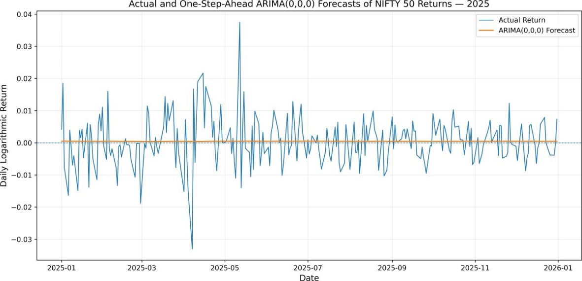
Figure 7:Actual and One-Step-Ahead ARIMA (0, 0, 0) Forecasts of NIFTY 50 Daily Logarithmic Returns During The 2025 Out-Of-Sample Period.
| Measure | Value |
|---|---|
| Number of forecasts | 249 |
| MAE | 0.005487 |
| RMSE | 0.007418 |
| Mean forecast error | -9.6E-05 |
| Directional accuracy | 50.20% |
Table 9: 2025 Out-Of-Sample Forecast Error Summary
These results are consistent with the diagnostics: although ARIMA (0, 0, 0) removes significant linear serial dependence from the conditional mean, daily return direction remains difficult to predict, with directional accuracy near the level expected from a non-informative forecast – so the evidence does not support strong linear predictability in daily NIFTY 50 returns. At the same time, the significant ARCH-LM results indicate this limited point-forecast performance should not be read as evidence of complete unpredictability: predictability in the conditional mean is weak, while the volatility process shows statistically significant temporal dependence.
ARIMA (0, 0, 0) is therefore retained as the parsimonious conditional-mean benchmark, with the significant ARCH effect motivating volatility-aware extensions discussed below.
DISCUSSION
The empirical findings present a coherent picture: a highly persistent price series yields a stationary return series after logarithmic transformation, whose weak linear dependence structure (correlation, stationarity, ACF/PACF evidence) explains the selection of the parsimonious ARIMA(0, 0, 0) specification, with Ljung–Box diagnostics confirming no significant remaining residual autocorrelation
However, this absence of linear autocorrelation is not evidence of constant variance: the highly significant ARCH-LM statistics, substantial excess kurtosis, and rejected residual normality together show that high- and low- volatility periods are not randomly distributed through time, consistent with the broader literature on conditional heteroskedasticity in equity index returns, including recent GARCH-based evidence for Indian markets and the foundational ARCH/GARCH framework [11,12,16,17].
The out-of-sample results reinforce this distinction: although ARIMA (0, 0, 0) achieves a small mean bias and marginally lower RMSE than the zero-return benchmark, its 50.20% directional accuracy indicates weak ability to anticipate individual daily return direction – broadly consistent with evidence that classical ARIMA provides a useful but limited benchmark relative to more flexible or nonlinear approaches, though the present study does not estimate such alternatives directly [7,10,25].
These findings carry an important implication: a model can be statistically adequate for the conditional mean while remaining an incomplete representation of the full return-generating process. Here, the principal forecastable component appears more likely associated with volatility dynamics than the direction of individual daily returns, supporting a cautious interpretation of ARIMA (0, 0, 0) as a transparent, parsimonious conditional-mean benchmark whose limited out-of-sample improvement suggests that more complex mean-equation specifications should not automatically be assumed superior.
From an applied perspective, investors and risk managers may obtain limited information from the expected value of the next daily return while facing substantial information content in the expected magnitude of future fluctuations. The significant ARCH effects therefore provide a clear empirical motivation for volatility-sensitive extensions: the NIFTY 50 forecasting problem should not be framed solely as predicting the next daily return, but should jointly consider the conditional mean and conditional variance, for which the present ARIMA results provide the necessary baseline.
CONCLUSION
This study examined the statistical characteristics and short-horizon forecast ability of the NIFTY 50 index using daily 2021–2025 observations, combining descriptive statistics, correlation analysis, logarithmic-return transformation, formal stationarity testing, ARIMA identification, residual diagnostics, and genuine out-of-sample forecasting, with particular attention to distinguishing conditional-mean predictability from conditional-variance dynamics.
The NIFTY 50 price level is highly persistent, while the logarithmic return series is stationary with a small mean, and reveals substantial departures from normality (full-sample skewness − 0.435115; excess kurtosis 4.394124), confirming that extreme daily movements occur more often than a Gaussian distribution would predict. Based on the ACF, PACF, and model selection evidence, ARIMA (0, 0, 0) provides a parsimonious conditional-mean representation, with Ljung–Box diagnostics confirming that the principal linear serial dependence has been adequately removed, so additional AR/MA terms would not be justified on residual-dependence grounds alone.
However, an adequate conditional-mean model does not imply an adequate representation of the full return-generating process: the highly significant ARCH-LM results and Jarque–Bera statistic (≈ 811.19) together indicate that although predictable linear dependence in the mean is limited, the magnitude of return innovations remains systematically time- varying. The genuine out-of-sample experiment (2021–2024 estimation; 249 observations from 2025 for evaluation) produced MAE = 0.00548694, RMSE = 0.00741835, mean forecast error ≈ − 0.00009617, and directional accuracy 50.20%; comparison with the zero-return benchmark (MAE 0.00546770, RMSE 0.00742496) shows economically small differences that do not support a claim of substantial improvement in daily point forecasting.
Taken together, the findings establish an important distinction between mean predictability and volatility predictability: there is little evidence that past daily returns contain sufficient linear information for materially superior short- horizon point forecasts, while the significant ARCH effects indicate systematic temporal structure in the conditional variance not captured by the constant-variance ARIMA specification. The study thus contributes a transparent empirical benchmark for NIFTY 50 return forecasting, indicating that the most important remaining structure lies outside the simple conditional mean equation – particularly relevant where forecasting the magnitude and risk of future market movements matters more than forecasting the exact direction of the next daily return.
PRACTICAL IMPLICATIONS AND RECOMMENDATIONS
ARIMA (0, 0, 0) is a useful baseline for the conditional mean of NIFTY 50 returns but not a complete forecasting framework. Correlation analysis is best used as an exploratory tool for market structure and price co- movement rather than a standalone forecasting method; statistical time series models applied to stationary return data are more appropriate for prediction, since they directly capture temporal dynamics. Trading volume is best used for assessing market activity and risk during volatile periods rather than predicting return direction. From a policy perspective, maintaining transparent, liquid, well-regulated markets remain important for market efficiency. The significant volatility dependence and non-Gaussian residual behaviour identified here provide strong empirical justification for extending the analysis to models that explicitly represent conditional variance dynamics.
LIMITATIONS AND DIRECTIONS FOR FUTURE RESEARCH
Three limitations should be acknowledged. First, the analysis relies primarily on univariate NIFTY 50 return information, excluding potentially informative variables such as macroeconomic indicators, interest rates, exchange rates, and global equity indices. Second, ARIMA models the conditional mean only and does not explicitly account for the significant conditional variance dynamics identified by the ARCH-LM tests. Third, the out of sample evaluation covers a single calendar year (2025), one economically relevant but finite window.
Future research should investigate volatility-sensitive models such as ARCH, GARCH, EGARCH, and GJR- GARCH [11,12], potentially combined with ARIMA mean equations, to jointly model the conditional mean and variance and more fully treat the volatility clustering identified here. Alternative error distributions, such as Student-t, should be considered given the substantial excess kurtosis observed. Further work could compare univariate models with multivariate and information-enriched frameworks, drawing on recent hybrid and nonlinear forecasting approaches [7,25], and could incorporate trading volume, macroeconomic and international market indicators, and rolling/expanding-window forecast evaluations to assess model stability across different market regimes.
Overall, the evidence suggests the principal challenge in modelling NIFTY 50 daily returns is not the absence of a statistically tractable conditional mean, but the presence of substantial time-varying volatility and non-Gaussian innovations. The ARIMA (0, 0, 0) results provide a useful baseline from which more sophisticated volatility and risk- forecasting models can be developed.
REFERENCES
- Securities and Exchange Board of India (2023). Annual Report 2022–23. SEBI, Mumbai.
- NSE Indices Limited (2024). Nifty 50 Whitepaper 2024. National Stock Exchange of India.
- Cont R. Empirical properties of asset returns: stylized facts and statistical issues. Quantitative finance. 2001;1(2):223. [Crossref] [Google Scholar]
- Tsay RS, Tsay RS. Analysis of financial time series. New York: wiley; 2010. [Crossref] [Google Scholar]
- Box GE, Jenkins GM, Reinsel GC, Ljung GM. Time series analysis: forecasting and control. John Wiley & Sons; 2015. [Crossref] [Google Scholar]
- Brooks C. STATA guide for introductory econometrics for finance. Cambridge university press; 2019. [Google Scholar]
- Stempień D, Ślepaczuk R. Hybrid models for financial forecasting: Combining econometric, machine learning, and deep learning models. 2505.19617. 2025. [Crossref] [Google Scholar]
- Hyndman RJ, Koehler AB. Another look at measures of forecast accuracy. International journal of forecasting. 2006;22(4):679-88. [Crossref] [Google Scholar]
- Diebold FX, Mariano RS. Comparing predictive accuracy. Journal of Business & economic statistics. 2002;20(1):134-44. [Crossref] [Google Scholar]
- Varshney S, Srivastava P. A comparative study of future stock price prediction through artificial neural network and ARIMA modelling. NMIMS Management Review. 2023;31(4):229-39. [Crossref] [Google Scholar]
- Engle RF. Autoregressive conditional heteroscedasticity with estimates of the variance of United Kingdom inflation. Econometrica: Journal of the econometric society. 1982:987-1007. [Crossref] [Google Scholar]
- Bollerslev T. Generalized autoregressive conditional heteroskedasticity. Journal of econometrics. 1986;31(3):307-27. [Crossref] [Google Scholar]
- Bollerslev T, Engle RF, Nelson DB. ARCH models. Handbook of econometrics. 1994;4:2959-3038. [Crossref] [Google Scholar]
- Nelson DB. Conditional heteroskedasticity in asset returns: A new approach. Econometrica: Journal of the econometric society. 1991:347-70. [Crossref] [Google Scholar]
- Engle RF, Ng VK. Measuring and testing the impact of news on volatility. The journal of finance. 1993;48(5):1749-78. [Crossref] [Google Scholar]
- Pinto P. Comparing the performance of GARCH family models in capturing stock market volatility in India. Shanlax International Journal of Management/Shanlax international journal of management. 2024. [Crossref] [Google Scholar]
- Mishra RR, Mishra S. Asymmetric Effects and Volatility Clustering in NSE NIFTY 50: A Comparative Analysis of GARCH Models. Asian Journal of Economics, Business and Accounting. 2024;24(11):142-52. [Crossref] [Google Scholar]
- Jain MK and Aggarwal S (2025). Decoding market cy-cles: A technical and time series analysis of Nifty 50. Jour-nal of Information Systems Engineering and Management, 10(50s). [Crossref]
- Kumar NP, Minithra R. Estimation of price volatility of Nifty 50 index using ADF and GARCH (1, 1). Indian Journal of Economics and Development. 2021;17(2):480-5. [Crossref] [Google Scholar]
- Vevek S, Selvam M, Sivaprakkash S. The persistence of volatility in Nifty 50. Indian Journal of Research in Capital Markets. 2022:8-18. [Crossref] [Google Scholar]
- Kaur P, Singla R. Modelling and forecasting Nifty 50 using hybrid ARIMA-GARCH Model. The Review of Finance and Banking. 2022;14(1):7-20. [Crossref] [Google Scholar]
- Mahajan V, Thakan S, Malik A. Modeling and forecasting the volatility of NIFTY 50 using GARCH and RNN models. Economies. 2022;10(5):102. [Crossref] [Google Scholar]
- Tejesh HR and Basha J (2023). Forecasting the Sensex and Nifty in-dices using ARIMA and GARCH models. MUDRA: Journal of Finance and Accounting, 10(1), 57–75. [Crossref]
- Bathia A, Padhy J, Tripathi MM, Balasubramaniam R, and Shah R (2024). Accuracy of ARIMA model for individual stocks of Nifty 50 – sector wise. European Economic Letters, 14(2), 3742–3765. [Crossref]
- Oukhouya H, Lmakri A, El Yahyaoui M, Guerbaz R, El Melhaoui S, Faizi M, et al. Predictive modeling for the Moroccan financial market: a nonlinear time series and deep learning approach. Future Business Journal. 2025;11(1):218.8. [Crossref] [Google Scholar]
- Investing com (2026). NIFTY 50 Historical Data. Investing.com Finan-cial Portal. Accessed 2026.
- Dickey DA, Fuller WA. Distribution of the estimators for autoregressive time series with a unit root. Journal of the American statistical association. 1979;74(366a):427-31. [Crossref] [Google Scholar]
- Kwiatkowski D, Phillips PC, Schmidt P, Shin Y. Testing the null hypothesis of stationarity against the alternative of a unit root: How sure are we that economic time series have a unit root?. Journal of econometrics. 1992;54(1-3):159-78. [Crossref] [Google Scholar]
- Akaike H. A new look at the statistical model identification. IEEE transactions on automatic control. 1974;19(6):716-23. [Crossref] [Google Scholar]
- Schwarz G. Estimating the dimension of a model. The annals of statistics. 1978:461-4. [Crossref] [Google Scholar]
- Ljung GM, Box GE. On a measure of lack of fit in time series models. Biometrika. 1978 ;65(2):297-303. [Crossref] [Google Scholar]
- Jarque CM, Bera AK. Efficient tests for normality, homoscedasticity and serial independence of regression residuals. Economics letters. 1980;6(3):255-9. [Crossref] [Google Scholar]

Article Processing Timeline
| 2-5 Days | Initial Quality & Plagiarism Check |
| 25-35 Days |
Peer Review Feedback |
| 45-60 Days | Total article processing time |
Why Publish with us?
Ethics & Policies
Editorial & Management
Useful Links
Journal Highlights
Open Access Journals
Journal of Psychiatry and Psychological Sciences
Journal of Cardiology and Heart Failure
Journal of Pediatric Medicine and Child Health
Journal of Nanoscience and Nanomaterials
Journal of Climate Change and Pollution
Journal of Molecular and Cellular Life Sciences
Journal of Plant Science and Biotechnology
Journal of Artificial Intelligence and Digital Health
Journal of Genomics and Precision Medicine
Journal of Robotics, Automation and Smart Systems
Journal of Sport Medicine, Science and Rehabilitation
Journal of Mathematics, Physics and Mechanics
Journal Flyer