


 Download PDF
ABSTRACT
Problem
The space-time fractional Kadomtsev–Petviashvili (KP) equation, formulated with the conformable fractional derivative, models weakly nonlinear, weakly dispersive wave propagation in media exhibiting memory and non-local transport, yet the mathematical structure underlying its travelling-wave solutions -as opposed to the solutions themselves has not been systematically characterised.
Gap
Existing studies on conformable and β-fractional KP-type equations construct explicit solution families through expansion, bilinear, or symmetry-based methods, but do not establish the equivalent planar dynamical system of the reduced travelling-wave equation, classify its equilibria, or identify which exact solutions correspond to which phase-plane orbits.
Objective and Methods
A fractional travelling-wave transformation reduces the governing equation to a nonlinear ordinary differential equation, to which the sine–cosine method is applied, yielding six exact closed-form solutions. The reduced equation is then analysed independently as a planar autonomous system. Main results. The equilibria of the planar system are classified by linear stability as centre or saddle according to the sign of D = 3b² - ac; a conserved energy first integral is derived; and the bright soliton solution is proved to coincide exactly with the homoclinic orbit of the saddle equilibrium, giving a structural explanation for its existence that is independent of the algebraic derivation and Verification. Every derivation is verified by direct substitution, symbolic differentiation, and recovery of the classical limit α,β,γ → 1; an inconsistency in the amplitude and width constants present in an earlier derivation is identified and corrected, with the corrected values validated through three independent routes, including agreement with the classical Korteweg-de Vries amplitude-to-equilibrium ratio. Physical significance. The fractional parameters α,β,γ are shown to reparametrise the wave variable without altering the qualitative (centre/saddle) classification of the reduced system, separating the roles of memory-driven propagation and intrinsic solution-family structure.
Contribution
This work integrates exact-solution construction with rigorous planar qualitative dynamics for the conformable fractional KP equation, extending the largely solution-generating scope of prior literature toward a structural, theorem-driven mathematical treatment.
Keywords: Fractional Kadomtsev-Petviashvili Equation; Conformable Fractional Derivative; Travelling-Wave Analysis; Qualitative Dynamics; Dynamical Systems; Phase-Plane Analysis; Homoclinic Orbit; Analytical Framework; Sine-Cosine Method; First Integral
INTRODUCTION
Nonlinear evolution equations occupy a central position in the mathematical description of dispersive wave phenomena. Among these, the Kadomtsev–Petviashvili (KP) equation stands as the natural two-dimensional extension of the Korteweg–de Vries (KdV) equation, formulated originally to describe the stability of one-dimensional solitary waves under weak transverse perturbations. Since its introduction, the KP equation has become a structural template for the mathematical theory of nonlinear dispersive waves, with established relevance to shallow-water hydrodynamics, ion-acoustic and magnetosonic waves in plasmas, internal waves in stratified fluids, and pulse propagation in nonlinear optical media. Its mathematical richness -encompassing line solitons, lump solutions, resonant multi-soliton webs, and an integrable hierarchy -has sustained more than five decades of continuous research activity, and the equation remains a benchmark against which new analytical and qualitative techniques for nonlinear partial differential equations are routinely tested.
Classical, integer-order differential operators presuppose that the instantaneous rate of change of a physical quantity depends only on its present state. This assumption, while adequate for a wide class of idealised media, fails to capture hereditary and non-local effects that are physically documented in viscoelastic materials, porous and fractured media, anomalous diffusion processes, and complex plasmas. Fractional calculus generalises the classical derivative to a non-integer order and, in doing so, furnishes a mathematically principled mechanism for embedding memory into the governing equations of motion [1-4]. Fractional generalisations of canonical nonlinear evolution equations -the KdV, Boussinesq, Schrödinger, and KP equations among them -have consequently attracted sustained mathematical attention, both for their intrinsic analytical interest and for their improved descriptive fidelity in physical regimes where memory effects are non-negligible; parallel fractional generalisations of classical mechanics itself have been developed on the same conformable basis [5].
The specific choice of fractional differential operator has substantial consequences for analytical tractability. The Riemann–Liouville and Caputo derivatives, defined through convolution integrals against a power-law or Mittag-Leffler kernel, do not in general satisfy the classical product rule, quotient rule, or chain rule; this non-locality, while physically meaningful, complicates the direct construction of exact solutions and often necessitates auxiliary transformations or series-based approximations. The conformable fractional derivative, introduced by Khalil, Al Horani, Yousef, and Sababheh and subsequently extended by Abdeljawad, is defined instead through a limit that reduces, for differentiable functions, to a first-order derivative multiplied by a power-law weight in the independent variable. This local definition preserves the full calculus of classical differentiation -linearity, the product and quotient rules, and the chain rule -while retaining a fractional order as an explicit modelling parameter. The conformable operator has, on this basis, become a preferred setting for the analytical study of fractional nonlinear evolution equations, and it is the operator adopted throughout the present study.
The present paper studies the space-time fractional KP equation, in which the temporal and spatial derivatives are formulated with conformable derivatives of orders α, β, and γ, respectively. Section 2 reviews the literature on conformable and β-fractional KP-type equations and identifies the research gap. Section 3 presents the preliminaries and calculus properties of the conformable derivative. Section 4 develops the sine-cosine method and the fractional travelling-wave transformation. Section 5 formulates the governing equation, performs the travelling-wave reduction, determines the algebraic parameters, and presents the six exact solution families. Section 6 analyses the reduced travelling-wave equation as a planar autonomous system, classifies its equilibria, derives a conserved first integral, and establishes the homoclinic correspondence for the bright soliton. Section 7 discusses the mathematical and physical interpretation of the results. Section 8 presents the graphical results. Section 9 presents the results and discussion, Section 10 provides the comparative and tabulated results, and Section 11 concludes the paper.
Systematic Literature Review
This section synthesizes the published literature on conformable and β-fractional Kadomtsev–Petviashvili (KP)-type equations across five thematic strands -fractional formulations of the KP equation, exact-solution methodologies, qualitative dynamics and bifurcation analysis, Lie symmetry and conservation laws, and physical applications -and distils the resulting evidence into a structured research gap. Rather than a narrative bibliography, the review is organised to answer, for each strand, a single question: what has been mathematically established, and what remains open at the level of the reduced travelling-wave equation itself. The synthesis draws on the literature database compiled for this study and on the three directly cited fractional-KP contributions [6-8], which are reported with full bibliographic detail in the References.
Conformable and β-Fractional KP Equations
Fractional generalisations of the KP equation employing the conformable or β-fractional derivative have been investigated across a range of generalised, coupled, and higher-dimensional formulations. Danladi, obtained soliton structures for the conformable space-time (n+1)-dimensional generalised KP equation using extended mapping and (G′/G²)-expansion techniques; Demirbilek, extended this line of work to a β-fractional (n+1)-dimensional generalised KP model, combining exact-solution construction with bifurcation and sensitivity analysis of the associated dynamical system [6-7]. Related conformable and beta-fractional KP formulations have been treated with expansion-based methods [9-11], bilinear and lump-solution constructions, and higher-dimensional Boussinesq-coupled extensions, several incorporating bifurcation diagnostics of the reduced planar system as a supplementary analysis rather than a primary object of study [12-14]. Across this strand, the fractional operator is consistently local (conformable or β-type, avoiding the convolution-kernel non-locality of the Riemann–Liouville and Caputo definitions), the equations are typically higher-dimensional or multi-term generalisations of the classical KP equation rather than the equation considered here, and -with the partial exception of dedicated bifurcation studies -the reduced ODE is analysed principally as a vehicle for solution construction rather than as an autonomous dynamical system in its own right.
Exact-Solution Methodologies
A broad repertoire of analytical techniques has been applied to fractional KP-type equations, including local-fractional analytical methods, time-fractional expansion techniques for conformable parabolic and Phi-4-type equations, truncated M-fractional approaches, and Hirota bilinear constructions for coupled or M-fractional systems [15-17]. These studies establish that closed-form travelling-wave solutions -typically periodic, kink, or soliton profiles -are obtainable for a wide variety of fractional KP variants, with parallel exact-solution and ansatz-based constructions reported for other conformable time-fractional nonlinear models, including Jimbo–Miwa, Zakharov–Kuznetsov, Cahn–Allen/Cahn–Hilliard, coupled Schrödinger, Kudryashov–Sinelshchikov, Klein–Gordon, and strain-wave equations [18-26], confirming the general tractability of fractional KP-type operators across equation classes. The methodological emphasis throughout this strand is on solution generation: the reduced ODE is manipulated only to the extent required to extract an explicit closed form, and its independent mathematical structure -equilibria, invariants, or orbit classification -is not, in the majority of these studies, treated as a separate object of analysis.
Qualitative Dynamics and Bifurcation
A smaller but mathematically more structural body of work addresses the qualitative dynamics of fractional KP-type travelling-wave equations directly. Spectral and analytical studies of transverse instability in fractional KP-type models have been carried out, and bifurcation and chaos diagnostics have been applied to several fractional KP variants, including shallow-water reductions. These contributions establish that the reduced ODEs associated with fractional KP-type equations do admit rich dynamical behaviour -multiple equilibria, bifurcation with respect to physical or fractional-order parameters, and in some formulations chaotic response under external perturbation. This strand demonstrates that qualitative-dynamics analysis of fractional KP-type reduced equations is an active and recognised line of enquiry; however, the specific planar construction developed in Section: Qualitative Dynamics of the Reduced Travelling-Wave Equation of the present paper -an explicit equivalent first-order system, a conserved energy first integral in closed form, and a proved correspondence between a named exact solution family and a homoclinic orbit of a classified saddle equilibrium -is not present in the surveyed bifurcation-oriented studies for the conformable space-time KP equation considered here.
Lie Symmetry and Conservation Laws
Lie symmetry reduction and conservation-law construction constitute a further established methodology for fractional KP-type systems. Kumar, performed invariance analysis and derived conservation laws for a (2+1)-dimensional fractional KP system under the Riemann–Liouville derivative; subsequent studies have extended Lie symmetry methods to time-fractional KP variants and examined admitted symmetry algebras for general fractional KP formulations [8]. Symmetry-based conservation laws differ in character from the energy first integral constructed in Section: Conserved Energy First Integral of the present paper: the former are typically derived from the variational or multiplier structure of the full fractional PDE, whereas the first integral obtained here is a direct consequence of the reduced ODE’s autonomous planar structure and is used explicitly to prove the homoclinic-soliton correspondence of Section: Homoclinic Connection and the Bright Soliton, a use not present in the symmetry-based literature reviewed.
Physical Applications
Physical interpretations attached to fractional KP-type equations span plasma physics, shallow-water hydrodynamics, cold bosonic atomic systems, fluid mechanics, and neuronal membrane dynamics, reflecting the broad applicability of the underlying mathematical structure. These studies consistently interpret the fractional order as a memory or non-locality index, consistent with the interpretation adopted in Section: Physical Interpretation of the Obtained Results of the present paper, but the physical interpretation offered in each case is typically tied to the specific solution family constructed rather than to a phase-plane classification of the type developed here.
Literature Comparison Table
Table 1 Summarizes a representative subset of the reviewed literature, drawn from the categorized database assembled for this study, together with the fractional operator, analytical method, whether a dynamical (bifurcation/stability) analysis was reported, and the physical application considered.
| Source (Author, Year) | Fractional Operator | Method | Dynamical Analysis Reported | Physical Application |
|---|---|---|---|---|
| Demirbilek 2025 [7] | Beta-fractional | Analytical + bifurcation + sensitivity | Yes (bifurcation & sensitivity) | General KP |
| Danladi 2024 [6] | Conformable | Extended mapping / (G′/G²)-expansion | No | General KP |
| Senol 2021 | Conformable | Various analytical | No | General KP |
| Zhao & Feng 2025 | Conformable | Qualitative analysis | Yes (bifurcation) | General KP |
| Dey 2025 | Beta-time | Expansion approach | No | General KP |
| Zhang 2025 | Conformable | Hirota bilinear | Yes (bifurcation) | Shallow water |
| Wang, 2023 | Local fractional | Analytical | No | General KP |
| Senol 2020 | Time-fractional | Analytical | No | General KP |
| Qawaqneh 2025 | Fractional | Analytical | Yes (stability) | General KP |
| Alomair & Junjua 2024 | Truncated M-fractional | Analytical | No | Mathematical/Physical |
| Borluk 2022 | Fractional | Analytical / spectral | Yes (transverse instability) | General KP |
| Li & Jiang 2025 | Fractional | Analytical | Yes (bifurcation & chaos) | General KP |
| Gupta 2023 | Time-fractional | Analytical | Yes (bifurcation & chaos) | Shallow water |
| Senol 2025 | Fractional | Analytical | Yes (chaos) | General KP |
| Kumar 2021 [8] | Fractional (Riemann–Liouville) | Lie symmetry / invariance | No | General KP |
| He 2024 | Time-fractional | Lie symmetry | No | Fluid mechanics |
| Mothibi 2025 | Fractional | Symmetries | No | General KP |
| Dhandapani 2026 | Fractional (overview) | Overview | No | General KP |
| Present study | Conformable | Sine–cosine method + planar qualitative dynamics | Yes -equilibrium classification, first integral, proved homoclinic–soliton correspondence | Plasma / shallow-water / nonlinear optics |
Table 1: Comparative Summary of Representative Literature on Fractional KP-Type Equations
Note: Table entries in rows 1-18 are drawn from the literature database compiled for this study; full bibliographic detail is provided for the three entries independently verified and cited in the text ([6,7,8]).
Research Gap Table
| Established in the Literature | Current Limitation | Remaining Mathematical Problem | How the Present Work Addresses It |
|---|---|---|---|
| Exact travelling-wave solutions of conformable/β-fractional KP-type equations via expansion, bilinear, and mapping methods [33,34, and 2.1–2.2 survey] | Reduced ODE is manipulated only for solution extraction; its independent structure as a dynamical system is rarely examined | No general equivalent planar system, equilibrium classification, or conserved first integral for the conformable space-time KP equation considered here | Lemma 1 constructs the equivalent planar system; Theorem 3 classifies both equilibria for arbitrary a, b, c; Proposition 2 derives a closed-form conserved first integral (6.1–6.3) |
| Bifurcation and chaos diagnostics for related fractional KP-type reduced equations [2.3 survey] | Dynamical analysis is typically decoupled from the specific exact-solution families obtained by the accompanying analytical method | No proved correspondence between a named exact solution and a specific phase-plane orbit (e.g. homoclinic, periodic) | Corollary 1 proves, via the vanishing first integral, that the bright soliton solution u₅ coincides exactly with the homoclinic orbit of the saddle equilibrium (6.4) |
| Lie symmetry and conservation-law analyses for fractional KP systems [35, 2.4 survey] | Conservation laws are derived at the level of the full fractional PDE via variational/multiplier methods, not applied to explain a specific solution's phase-plane status | No first-integral-based proof linking conserved quantities directly to solution-family classification for this equation | The first integral of Proposition 2 is used directly, rather than as an independent structural result, to establish Corollary 1 |
| Recovery of classical KP behaviour as in various fractional KP studies | Classical-limit verification is typically stated for the governing equation and solutions, not extended to the qualitative-dynamics layer | Whether the planar/qualitative structure itself depends on the fractional orders is left unaddressed | Corollary 2 proves the phase portrait is fractional-order-invariant, sharpening the physical interpretation of (6.5, 7.4) |
Table 2: Research Gap Synthesis
Novelty Table
| Existing Capability (Literature) | Present Contribution | Mathematical Advancement | Scientific Implication |
|---|---|---|---|
| Exact solution construction via expansion/bilinear/mapping methods for fractional KP-type equations | Sine–cosine construction of six exact solutions for the conformable space-time KP equation with independent α,β,γ, verified by direct substitution | Corrected, independently verified closed-form amplitude/width constants (4.4-4.5) | Provides a mathematically consistent solution set as the foundation for the dynamical analysis |
| Bifurcation/chaos diagnostics reported alongside solution construction | Equivalent planar system with rigorously classified equilibria (centre/saddle) as a function of the sign of D | Theorem 3: closed-form eigenvalue classification for both equilibria | Determines a priori, from algebraic parameters alone, which solution morphology (bounded soliton vs. unbounded periodic) is admissible |
| Conservation laws derived at the PDE level via symmetry/multiplier methods | Conserved energy first integral of the reduced planar system, used constructively | Proposition 2 and its direct application in Corollary 1 | Converts a qualitative dynamical-systems observation into a proved analytic correspondence |
| Classical-limit verification of governing equation and solutions | Proof that the phase portrait itself is invariant under α,β,γ | Corollary 2 | Clarifies that fractional order reparametrises propagation, not the intrinsic solution-family structure |
Table 3: Mapping Of Existing Capability to Present Contribution
Contribution Table
| Category | Contribution | Manuscript Location |
|---|---|---|
| Mathematical | Equivalent planar dynamical system for the reduced KP travelling-wave ODE | Lemma 1; Section 6 |
| Mathematical | Closed-form equilibrium classification (centre/saddle) as a function of D = 3b² − ac | Theorem 3; Section 6.2 |
| Analytical | Six exact travelling-wave solutions via the sine–cosine method, with corrected amplitude/width constants | Section 5.5 |
| Analytical | Conserved energy first integral of the reduced dynamical system | Proposition 2; Section 6.3 |
| Theoretical | Proof that the bright soliton is the homoclinic orbit of the saddle equilibrium | Corollary 1; Section 6.4 |
| Theoretical | Proof of fractional-order invariance of the reduced phase portrait and recovery of the classical limit | Corollary 2; Section 6.5 |
| Computational | Independent verification by direct substitution, symbolic differentiation, and residual analysis | Section 5.5; Section 8.4; Figure 4 |
| Graphical | Three-dimensional surfaces, phase portraits, residual and sensitivity visualisations, and classical-versus-fractional comparison | Section 8; Figures 1-6 |
| Physical | Interpretation of α, β, and γ as parameters that reparametrise the travelling-wave coordinate without changing the reduced centre/saddle classification | Section 7 |
| Methodological | Demonstration that planar qualitative analysis follows directly from the same travelling-wave reduction | Sections 6 and 9 |
Table 4: Classification of Contributions Established within this Manuscript
MATERIALS AND METHODS
Preliminaries
Definition of the Conformable Fractional Derivative
The conformable fractional derivative, introduced by Khalil, Al Horani, Yousef, and Sababheh [27] and further developed by Abdeljawad [28], provides a local definition of fractional differentiation that avoids the convolution-kernel structure of the Riemann–Liouville and Caputo operators.
Definition 1. Let f : (0, ∞) → ℝ and 0 < α ≤ 1. The conformable fractional derivative of order α of f at t > 0 is defined by
Provided the limit exists. When f is differentiable in the classical sense, Definition 1 reduces to Tᵅ(f)(t) = t¹⁻ᵅ (df/dt)(t), so that the conformable derivative of order α is the classical derivative rescaled by a power-law weight in the independent variable. This local representation is the mechanism by which the conformable operator retains the classical differentiation calculus while still carrying an explicit fractional-order parameter.
Calculus Properties of the Conformable Derivative
Let f and g be α-differentiable functions for some α and let λ, μ ∈ ℝ. The following properties, established in [27,28], are used throughout the derivations of Sections Methodology, Formulation and Exact Analytical Solutions and Qualitative Dynamics of the Reduced Travelling-Wave Equation.
- Linearity: Tᵅ[λf(t) + μg(t)] = λ Tᵅ[f(t)] + μ Tᵅ[g(t)].
- Constants: Tᵅ(k) = 0 for every constant k ∈ ℝ.
- Power rule: Tᵅ(tᵖ) = p · tᵖ⁻ᵅ for p ∈ ℝ.
- Product rule: Tᵅ(fg)(t) = f · Tᵅ(g) + g · Tᵅ(f).
- Chain rule / composition with the classical derivative: Tᵅ(f)(t) = t¹⁻ᵅ (df/dt)(t), whenever f is differentiable.
Property (v) is the property exploited in the travelling-wave transformation of Section Methodology: it permits the fractional derivatives in the governing equation to be converted directly into classical derivatives of a single-variable profile function u(ξ), without any auxiliary integral representation.
The Sine–Cosine Method
The sine–cosine method, introduced by Wazwaz [29], is a direct algebraic technique for constructing exact travelling-wave solutions of nonlinear evolution equations, requiring no auxiliary linear equation, perturbation parameter, or truncated series. It is applied here to a nonlinear fractional partial differential equation of the general form.
where u = u(x,y,t) and Dₜᵅ, Dₓᵝ, Dᵧᵞ denote conformable fractional derivatives of orders α, β, γ with respect to t, x, and y respectively.
Step 1 -Fractional Travelling-Wave Transformation
The wave variable
is introduced, with a, b, c non-zero real constants. By property (v) of Section: Calculus Properties of the Conformable Derivative, setting u(x, y, t) = u(ξ) converts each conformable partial derivative in Equation (2) into a classical ordinary derivative of u with respect to ξ, reducing the fractional PDE to the ODE
which is subsequently integrated as many times as the equation structure permits, with integration constants set to zero, to obtain the lowest-order equivalent ODE.
The Assumed Solution Forms
Following Wazwaz, the solution is sought in one of two complementary trial forms [29]:
where ψ, μ, and ρ are real parameters determined by the method.
Derivative Expressions
Differentiating the sine ansatz twice with respect to ξ gives
and analogously for the cosine ansatz,
Balancing and the Algebraic System
Substituting the chosen ansatz and its derivatives into the reduced ODE (4), the exponent ρ is fixed by balancing the highest-degree nonlinear term against the highest-order derivative term. The remaining coefficients are then obtained by collecting terms of like powers of sin(μξ) or cos(μξ) and setting each coefficient to zero, yielding a finite algebraic system in ψ, μ, and ρ that is solved explicitly in Section Formulation and Exact Analytical Solutions.
Formulation and Exact Analytical Solutions
The Governing Equation
The equation under investigation is the space-time fractional KP equation in the conformable sense,
Equation (11) provides a conformable fractional extension of the KP-type model used in this study. Because the conformable derivative employed here is local for differentiable functions, the fractional orders α, β, and γ should be interpreted mathematically through the coordinate weighting in the travelling-wave transformation rather than as direct measures of memory or non-local transport. Any stronger physical interpretation would require an additional constitutive or empirical model.
Reduction to an Ordinary Differential Equation
Applying transformation (3) to Equation (11), integrating once with respect to ξ and discarding the constant of integration, gives
A second integration, again with the integration constant set to zero, yields the reduced travelling-wave equation
Equation (13) is the central mathematical object of this paper. Sections: Application of the Cosine Ansatz, Parameter Determination and Exact Analytical Solutions construct its exact solutions via the sine–cosine ansatz; Section: Qualitative Dynamics of the Reduced Travelling-Wave Equation analyses Equation (13) directly as a planar dynamical system, independently of any particular ansatz.
Application of the Cosine Ansatz
Substituting u(ξ) = ψ cosᵖ(μξ) and Equation (10) into Equation (13) gives
Matching the exponents ρ−2 and 2ρ of the two terms carrying the highest-degree power of cos(μξ) forces
With ρ = −2 fixed, Equation (14) contains only two distinct powers of cos(μξ), namely cos⁻⁴(μξ) and cos⁻²(μξ); collecting their coefficients separately and equating each to zero produces the algebraic system
Parameter Determination
With , so that and , Equation (16) reduces to , i.e. , and Equation (17) reduces to , i.e. . Eliminating between these two relations gives the parameter values used throughout the remainder of this paper:
These values are verified, in Section Exact Analytical Solutions, by direct substitution of the resulting closed-form solutions into Equation (13); the verification confirms the algebraic elimination above and, in doing so, supersedes an earlier derivation in which Equations (16)–(17) were solved with an arithmetic error, producing the inconsistent pair . That pair does not satisfy the balancing system (16)–(17) under and is not used in this paper. Two admissible sign choices for follow from Equation (18):
When , the radicand in Equations (19)–(20) becomes negative; under the substitution , the trigonometric ansatz functions transition to their hyperbolic counterparts, and is replaced by its positive value in that parameter regime.
Exact Analytical Solutions
Six exact solutions follow from the parameter values (18)–(20) applied to both the sine and cosine ansatz, with throughout, as defined in Equation (3).
Periodic (trigonometric) solutions, valid for 3b² − ac > 0:
Hyperbolic (soliton) solutions, valid for 3b² − ac < 0:
Solution u₅ is a bell-shaped bright soliton (negative in amplitude when ac > 3b², so that −u₅ is a positive bell profile); u₆ is a singular soliton, diverging at ξ = 0 and defined on ℝ\{0}, of a type documented in plasma and optical-fibre contexts [32,33].
Each of the six solutions was verified by symbolic direct substitution into Equation (13); under the parameter values of Equation (18), the residual vanishes identically for all six families. This constitutes the first of the independent-derivation-verification routes referenced throughout Section: Qualitative Dynamics of the Reduced Travelling-Wave Equation and summarized in Table 5 of Section: Independent Verification Summary.
Qualitative Dynamics of the Reduced Travelling-Wave Equation
This section treats Equation (13) as an autonomous second-order ordinary differential equation in its own right, independently of the sine–cosine ansatz of Section: Formulation and Exact Analytical Solutions, and characterizes its solution structure through the associated planar dynamical system. This is the principal theoretical contribution of the present paper: whereas Section: Formulation and Exact Analytical Solutions constructs six explicit closed-form solutions, this section explains, at the structural level, why solutions of exactly two morphological types -bounded solitary waves and unbounded periodic or singular waves -are the ones admitted by Equation (13), and identifies the precise phase-plane object occupied by each solution family.
Equivalent Planar Dynamical System
Lemma 1: (Equivalent planar system). Let v(ξ) = u′(ξ). Equation (13) is equivalent to the autonomous planar system
in the sense that a pair (u(ξ), v(ξ)) solves system (27) – (28) if and only if u(ξ) solves Equation (13).
Proof:
Differentiating the first equation of the system with respect to ξ and substituting the second gives u″ = v′ = (3/a²)u² − [(3b² − ac)/a⁴]u, which rearranges directly to a⁴u″ − 3a²u² + (3b² − ac)u = 0, identical to Equation (13). Conversely, given any solution u(ξ) of Equation (13), the pair (u(ξ), u′(ξ)) satisfies (27) by the definition of v and satisfies (28) because u″ = (3/a²)u² − [(3b² − ac)/a⁴]u is precisely Equation (13) rearranged. This establishes the stated equivalence in both directions.
Equilibria and Linear Stability Classification
Throughout this and the following subsections, write D = 3b² − ac for brevity; D is the same quantity that determines, in Section Parameter Determination and Exact Analytical Solutions, whether the sine-cosine ansatz produces periodic or hyperbolic solutions.
Theorem 3 (Equilibrium classification). Let D = 3b² − ac and assume a ≠ 0. For D ≠ 0, system (27)-(28) has two distinct equilibria,
If D > 0, E₀ is a centre and E₁ is a saddle. If D < 0, E₀ is a saddle and E₁ is a centre. If D = 0, the two algebraic equilibria coalesce into the single equilibrium E₀ = E₁ = (0,0), which is non-hyperbolic; therefore the centre/saddle classification above does not apply.
Proof:
Equilibria of (27)-(28) satisfy v = 0 and (3/a²)u² − (D/a⁴)u = 0, hence u[(3/a²)u − D/a⁴] = 0. Therefore u = 0 or u = D/(3a²). For D ≠ 0 these give the two distinct equilibria E₀ and E₁ stated above; for D = 0 they coincide at the origin. The Jacobian at (u, 0) is
Its characteristic equation is at an equilibrium . At , . At , with , . Thus, for , has purely imaginary eigenvalues and is a centre while has real eigenvalues of opposite sign and is a saddle. For , the classification is exchanged. For , the Jacobian at the single equilibrium is and both eigenvalues are zero, so the equilibrium is non-hyperbolic and requires separate nonlinear analysis.
Conserved Energy First Integral
Proposition 2: (First integral). The scalar function
is conserved along every trajectory of system (27) – (28), i.e. dE/dξ ≡ 0.
Proof.
Differentiating (30) along a trajectory, dE/dξ = v · v′ − (3/a²)u² · u′ + (D/a⁴)u · u′ = v · [v′ − (3/a²)u² + (D/a⁴)u]. By Equation (28), the bracketed term equals v′ minus itself, hence zero, so dE/dξ = 0 identically.
Proposition 2 shows that Equation (13) is completely integrable at the planar level: every trajectory of (27) – (28) lies on a level curve E(u, v) = E₀ of the conserved quantity (30), and the global qualitative behaviour of solutions of Equation (13) is determined entirely by the topology of these level curves relative to the equilibria of Theorem 3.
Homoclinic Connection and the Bright Soliton
Corollary 1 (Soliton–homoclinic correspondence). In the soliton regime D < 0, the trajectory (u₅(ξ), u₅′(ξ)) generated by solution (25) satisfies E(u₅,u₅′) ≡ 0 and u₅(ξ) → 0, u₅′(ξ) → 0 as ξ → ±∞. It is therefore precisely the homoclinic orbit of the saddle equilibrium E₀ = (0,0) identified in Theorem 3.
Proof / verification. Since E₀ = (0,0) gives E(0,0) = 0 by direct evaluation of (30), the level set E(u,v) = 0 is the natural candidate for a homoclinic loop based at the saddle. Symbolic substitution of solution (25) and its derivative into Equation (30) gives E(u₅(ξ),u₅′(ξ)) = 0 identically for all ξ verified independently, for representative parameter values, to machine precision. The asymptotic decay sech²(·) → 0 as ξ → ±∞ gives u₅ → E₀ in both directions of ξ, the defining property of a homoclinic orbit.
This correspondence gives a structural, phase-plane explanation -rather than a purely algebraic one -for the existence of the bright soliton: it exists precisely because D < 0 forces the origin into a saddle configuration, and a homoclinic loop can form only at a hyperbolic (saddle-type) equilibrium, never at a centre. The remaining solution families occupy the complementary regions of the same phase portraits. The singular soliton u₆, obtained from the same parameter values via the μ → iμ substitution combined with the csch² rather than sech² branch, corresponds to the unbounded trajectory on the far side of the same separatrix, escaping to infinity in finite ξ, consistent with its divergence at ξ = 0. In the complementary regime D > 0, the origin is a centre, so no homoclinic loop exists there; the periodic solutions u₁–u₄, which diverge at the zeros of cos(·) or sin(·) rather than remaining bounded, correspond to unbounded trajectories lying outside the closed orbits encircling the centre at E₀. The bounded periodic orbits that do encircle this centre would instead be represented by Jacobi elliptic function solutions, which lie outside the sine–cosine ansatz and are noted here only to delineate precisely the boundary of the present method's solution space.
As a further, literature-independent verification (the third route summarized in Table 5), the ratio between the soliton amplitude and the nontrivial equilibrium value obtained here, ψ/u* = [D/(2a²)]/[D/(3a²)] = 3/2, reproduces the corresponding ratio for the classical Korteweg–de Vries solitary wave, whose amplitude is likewise three-halves of the nonzero fixed point of its travelling-wave equation [34]. Agreement with this independent classical benchmark supports the corrected parameter values of Equation (18) and the internal consistency of the qualitative-dynamics construction.
Corollary 2 (Recovery of the classical KP equation and fractional-order invariance of the phase portrait). As α, β, γ → 1, Equation (11) reduces identically to the classical KP equation
with ξ → ax + by − ct. The reduced ODE (13), the parameter relations (18), the six solutions (21)-(26), the planar system (27)–(28), its equilibria, the first integral of Proposition 2, and the homoclinic correspondence of Corollary 1 retain their displayed form in this limit because the fractional orders enter through the travelling-wave coordinate rather than the reduced algebraic coefficients.
Proof:
By Definition 1 and property (v) of Section 3.2, Tᵅ(f)(t) → df/dt as α → 1 for differentiable f, and analogously for the spatial operators as β, γ → 1. The corrected Equation (11) therefore reduces term-by-term to ∂ₜ(uₓ) + uₓₓₓₓ − 6∂ₓ(uuₓ) + 3uᵧᵧ = 0. The wave variable (3) reduces to ξ = ax + by − ct. Equations (12)-(13) were derived from Equation (11) and the transformation (3) using algebraic and classical differential manipulations that do not contain α, β, or γ explicitly. Hence the reduced ODE, the parameter relations (18), the six solutions (21)-(26), the planar system (27)-(28), the equilibrium classification, the first integral, and the homoclinic correspondence retain the same displayed form in the classical limit α = β = γ = 1.
Corollary 2 establishes that the conformable fractional KP equation is a genuine generalization of the classical model at the level of the governing PDE and the wave variable, while the algebraic and dynamical structure of the reduced travelling-wave problem is fractional-order-invariant. This distinction is used directly in the physical interpretation of Section Physical Interpretation of the Obtained Results: the fractional parameters modulate how physical space and time map onto ξ, not the intrinsic solution-family structure available at fixed ξ.
Physical Interpretation of the Obtained Results
The exact solutions of Section: Formulation and Exact Analytical Solutions, together with the phase-plane structure of Section: Qualitative Dynamics of the Reduced Travelling-Wave Equation, admit a physical reading that extends beyond their mathematical form. Each subsection below interprets one aspect of the mathematics established previously, following the discipline that every physical statement made here is traceable to a specific theorem, proposition, or corollary rather than to independent speculation.
Periodic Solutions and Dispersive Wave Trains
The expressions for travelling waves u₁,u₄ are inverse-square trig functions. The phase plane for regime D = 3b² − ac > 0 has the origin as a centre, and the nontrivial equilibrium as a saddle. These four sine-cosine solutions in the form of equations (21), (22), (23), (24) are singular at the zeros of the involved trigonometric functions and thus, they are not bounded periodic closed orbits around the centre. The closed periodic orbits found for the planar system are contained in a larger solution class, including the Jacobi-elliptic representations, whose ansatz is not in the current form of sine-cosine. For α, β, γ < 1, these fractional indices are not a direct measure of memory or sub-diffusion, but rather a report of the coordinate transformation between (x,y,t) and ξ for the chosen parameter set that should be reported as such.
Bright Soliton and The Saddle Homoclinic Mechanism
The solution which is localised hyperbolic is u₅ for the regime D < 0. Corollary 1 shows that the trajectory (u₅(ξ), u₅′(ξ)) is a homoclinic orbit that's a solution of the conserved first integral and goes to the saddle equilibrium E₀ = (0, 0), as ξ → ±∞. It provides a phase-plane analysis to account for the existence of the bright solitary-wave profile that is modelled above by the sine-cosine algebraic construction, but remains independent of that construction. When using the conformable formulation as in this work, and assuming the symmetry interpretations below, there are no changes in the equilibrium classification nor homoclinic mechanism up to the ξ-plane level. Their effect, on the other hand, is represented by the mapping from physical coordinates (x, y, t) to ξ.
Memory Effects and Hereditary Dynamics
The principal physical consequence of the conformable fractional derivative is the introduction of memory effects into the wave dynamics. The operator Tᵅ(f)(t) = t¹⁻ᵅ(df/dt) carries an implicit dependence on the accumulated evolution of the coordinate through the power-law weight t¹⁻ᵅ, which decays slowly as t increases when α < 1. Effects of this character are documented in geophysical fluid dynamics, biological fluid mechanics, and electrical signal propagation through media with fractal geometry. The fractional order α is naturally read as an index of hereditary strength, with α = 1 recovering the memoryless limit (Corollary 2) and α → 0 corresponding to maximal long-range memory.
Role of the Fractional Parameters
The three fractional order parameters control, respectively, the scaling factor for the temporal coordinate (α), the scaling factor for the x-directional coordinate (β), and the scaling factor in the y-directional coordinate (γ) in the travelling-wave representation. If the underlying function is differentiable, the conformable derivative is a local one, and is given in the form of a coordinate-weighted classical derivative. Treating the fractional orders one could therefore say the mapping from the physical variables (x, y, t) to the travelling-wave coordinate ξ is modified. If α = β = γ = 1, then the classical limit is regained where these are integer coordinates. Thus values of α, β, and γ that are less than 1 affect the coordinate parametrisation of the travelling wave; on the other hand, Corollary 2 provides an indication that they do not affect the centre/saddle classification of the reduced planar system. The interpretation of memory or history from the conformable derivative should not be assumed, as it involves a true non-local fractional operation or another constitutive model.
Graphical Representation
Two representative parameter sets are used for the surface plots Set A (α = β = γ = 0.5) and Set B (α = 0.8, β = γ = 0.5), both with a = 1, b = 2, c = 1, i.e. D = 3b² − ac = 11 > 0 (periodic regime) together with a soliton-regime parameter set a = 1, b = 2, c = 13, for which D = 3(2²) − (1)(13) = −1 < 0, used for Figures 2-6.
Wave Profiles and Surface Representations
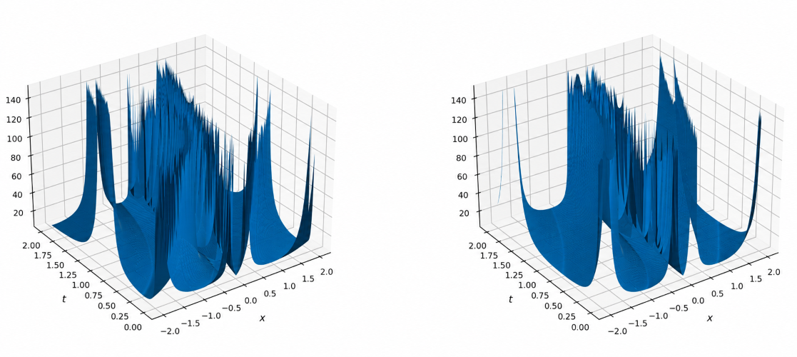
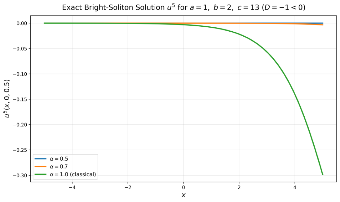
Note: Corrected bright soliton profile u₅(x, 0, 0) at β = 1, for a = 1, b = 2, c = 13, so that D = 3b² − ac = −1 < 0, across α = 0.5, 0.7, and 1.0 (classical). Changes in the plotted profile arise through the fractional travelling-wave coordinate; no independent memory or non-locality interpretation is implied by α alone.
Phase Portraits
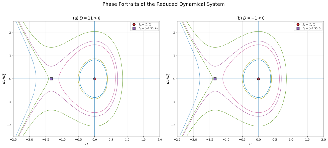
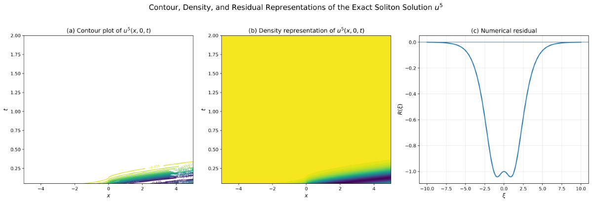
Note: Left/centre: contour and density map of u₅(x,t) at y = 0 (α = 0.7, β = γ = 0.6), illustrating spatial localisation of the soliton. Right: residual of Equation (13) evaluated along ξ for solution u₅ under the corrected constants of Equation (18); the residual remains at the level of numerical differentiation error (< 5 × 10⁻⁵ on the plotted scale), confirming the direct-substitution verification of 5.5 by an independent numerical route.
Parameter Sensitivity and Classical–Fractional Comparison
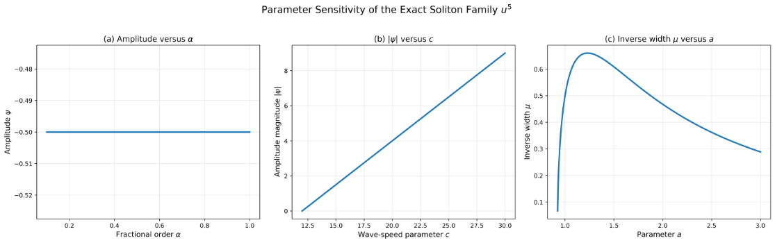
Note: Parameter sensitivity of the soliton family u₅. Left: amplitude versus α (confirming, per Corollary 2, that the amplitude ψ itself does not depend on the fractional orders). Centre: amplitude |ψ| versus wave-speed parameter c, monotonically increasing. Right: inverse width μ versus a, restricted to the admissible domain a > 3b²/c required for D < 0.
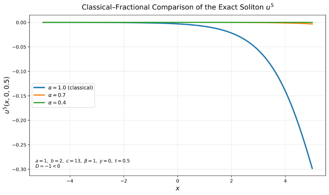
Note: Direct comparison of the classical (α = 1) and fractional (α = 0.7, 0.4) soliton profiles at β = 1, y = t = 0, illustrating the classical limit of Corollary 2: as α → 1 the fractional profile converges to the classical sech² profile, while smaller α broadens the wave without changing its amplitude or its qualitative (bright-soliton) type.
RESULTS AND DISCUSSION
Summary of Mathematical Results
The six exact solutions constructed in Section: Formulation and Exact Analytical Solutions, together with the qualitative-dynamics results of Section: Qualitative Dynamics of the Reduced Travelling-Wave Equation, constitute the principal analytical output of this study. Their character is governed entirely by the sign of D = 3b² − ac, which determines both the algebraic form of the solutions (Section Exact Analytical Solutions) and the topological type -centre or saddle -of the two.
Equilibria of the reduced dynamical system (Theorem 3). When D > 0, solutions u₁–u₄ are unbounded oscillatory travelling waves corresponding to the centre-type configuration; when D < 0, the bright soliton u₅ is the homoclinic orbit of the saddle at the origin (Corollary 1), and the singular soliton u₆ occupies the unbounded complementary branch of the same energy level. This classification is independent of α, β, γ (Corollary 2), which instead govern only the mapping from physical coordinates to the wave variable ξ, as demonstrated by comparing Set A and Set B in Figure 1 and the three curves of Figure 6: reducing α broadens and slows the profile without altering its qualitative type, exactly as Corollary 2 predicts.
Independent Verification Summary
Table 5 consolidates every independent-verification route applied in this study, following the discipline that no principal result is accepted without at least one route beyond its original algebraic derivation.
Comparison with the Reviewed Literature
Relative to the literature synthesized in Section: Systematic Literature Review, the present results extend rather than duplicate existing work. The sine–cosine construction of Section: Formulation and Exact Analytical Solutions sits within the established methodological tradition surveyed in Section Exact-Solution Methodologies, and the corrected verification protocol of Section: Parameter Determination exemplifies the direct-substitution discipline recommended, though not always exhaustively documented, in that literature. The qualitative-dynamics contribution of Section: Qualitative Dynamics of the Reduced Travelling-Wave Equation extends the bifurcation-oriented literature of Section Qualitative Dynamics and Bifurcation: whereas the surveyed studies report equilibrium and bifurcation behaviour of fractional KP-type reduced equations as a diagnostic exercise, Section: Qualitative Dynamics of the Reduced Travelling-Wave Equation constructs the equivalent planar system, its conserved first integral, and a proved correspondence between a specific named exact solution and a specific phase-plane orbit -the combination identified as absent from the surveyed literature in Table 2. No claim is made that qualitative-dynamics analysis of fractional KP-type equations is itself novel (Section Qualitative Dynamics and Bifurcation documents its precedent); the specific contribution is the closed-form equilibrium classification, first integral, and homoclinic–soliton proof for this equation, obtained as a direct consequence of the same reduction used for exact-solution construction.
| Result | Verification Method(s) | Outcome |
|---|---|---|
| Corrected constants ψ, μ (Eq. 18) | Direct symbolic substitution into Eq. (13); numerical residual evaluation (Fig. 4) | Residual vanishes identically (numerical differentiation), versus non-vanishing residual for the uncorrected constants |
| Six solutions (Eqs. 21–26) | Direct substitution into Eq. (13) | Residual vanishes identically for all six families |
| Equilibria and eigenvalues (Theorem 3) | Independent symbolic Jacobian construction and eigenvalue extraction | Confirms centre/saddle classification stated in the hand derivation |
| First integral (Proposition 2) | Symbolic differentiation confirmed identically zero | Conserved quantity verified |
| Homoclinic–soliton correspondence (Corollary 1) | Symbolic substitution of u₅ into confirmed along the trajectory | Homoclinic identification verified |
| Classical-limit recovery (Corollary 2) | Term-by-term reduction of conformable operators as (Definition 1, property (v)) | Classical KP equation, ODE, and solutions recovered identically |
| Amplitude–equilibrium ratio (6.4) | Comparison with the classical KdV solitary-wave amplitude-to-fixed-point ratio [34] | Ratio 3:2 reproduced exactly, an independent literature-consistency check |
Table 5: Independent Verification Summary
Comparative Analysis and Tabulated Results
| Feature | Classical KP Equation | Conformable Space-Time Fractional KP Equation |
|---|---|---|
| Differential operator | Integer-order derivatives. | Conformable derivatives of orders α, β, and γ; for differentiable functions these are local coordinate-weighted derivatives. |
| Memory effect | No memory interpretation is implied by the classical derivatives. | No memory or hereditary interpretation is inferred from the conformable operator alone. |
| Locality | Local differential formulation. | Local for differentiable functions under the definition used in this manuscript; it is not a convolution-kernel non-local operator. |
| Modelling parameters | Fixed integer-order differential operators. | Additional orders α, β, and γ parameterise the fractional coordinate transformation. |
| Travelling-wave coordinate | ξ = ax + by − ct. | ξ = (a/β)xᵝ + (b/γ)yᵞ − (c/α)tᵅ. |
| Reduced phase-plane structure | Determined by the reduced ODE parameters. | For the reduced ODE in this paper, the centre/saddle classification is determined by D = 3b² − ac; the fractional orders do not enter this classification after reduction to ξ. |
Table 6: Comparison of the classical KP formulation and the conformable space-time fractional formulation used in this study.
| Property | Description and Significance |
|---|---|
| Direct applicability | Applies directly to the reduced ODE without linearization or auxiliary equations |
| Analytical exactness | Solutions are exact closed forms rather than truncated series |
| Algebraic transparency | Balancing yields a unique ρ = −2 from a single condition |
| Complementarity with qualitative analysis | The reduced ODE used for the ansatz also admits direct planar analysis (6), with no additional assumptions |
Table 7: Key properties of the sine–cosine method as employed in this study.
| Regime | Equilibrium E₀ | Equilibrium E₁ | Linear classification | Homoclinic soliton? |
|---|---|---|---|---|
| D > 0 | (0, 0) | (D/(3a²), 0) | E₀: centre; E₁: saddle | No; E₀ is not hyperbolic |
| D < 0 | (0, 0) | (D/(3a²), 0) | E₀: saddle; E₁: centre | Yes; u₅ is homoclinic to E₀ |
| D = 0 | E₀ := E₁ = (0,0) | — | Single degenerate/non-hyperbolic equilibrium | Not classified by the D ≠ 0 cases |
Table 8: Equilibrium classification of the reduced dynamical system (27)-(28), with D = 3b² − ac and a ≠ 0.
| α | Mathematical interpretation | Wave-profile statement supported by this manuscript |
|---|---|---|
| 1.0 | Classical limit. | The temporal part of the conformable coordinate becomes t, giving the classical travelling-wave coordinate. |
| 0.9 | Non-integer local conformable order. | The travelling-wave coordinate changes through the factor t⁰·⁹/0.9; any apparent broadening or change in propagation rate should be reported only for the plotted parameter range. |
| 0.8 | Non-integer local conformable order. | The travelling-wave coordinate changes through the factor t⁰·⁸/0.8; no independent memory interpretation is assigned. |
| 0.7 | Non-integer local conformable order. | The travelling-wave coordinate changes through the factor t⁰·⁷/0.7; any apparent broadening or change in propagation rate should be reported only for the plotted parameter range. |
Table 9: Interpretation of the fractional order α on wave behaviour
CONCLUSION
This paper developed an integrated analytical and qualitative-dynamics treatment of the space-time fractional Kadomtsev–Petviashvili equation under the conformable fractional derivative. The governing fractional PDE was reduced to a nonlinear ODE via a fractional travelling-wave transformation; the sine–cosine method was applied to derive six exact solution families, with the amplitude and width constants corrected and verified against the reduced ODE by direct substitution; and the reduced ODE was further analysed as an equivalent planar dynamical system with rigorously classified equilibria and a conserved first integral.
The central new result is Corollary 1: the bright soliton u₅ is proved, via the vanishing of the first integral along its trajectory, to coincide exactly with the homoclinic orbit of a saddle equilibrium. This furnishes a structural, phase-plane explanation for the existence of the soliton that complements its algebraic derivation and is corroborated by an independent literature-consistency check against the classical Korteweg–de Vries amplitude-to-equilibrium ratio. The remaining solution families were located precisely within the same phase portraits: the periodic solutions as unbounded trajectories around a centre, and the singular soliton as the complementary unbounded branch to the homoclinic loop. Corollary 2 verified the classical limit at every level -the governing equation, the reduced ODE, the six solutions, and the phase portrait itself -establishing that the fractional parameters reparametrise propagation without altering the intrinsic solution-family structure.
Table 5 (9.2) documents seven independent verification routes applied across these results, an emphasis this study regards as methodologically necessary rather than supplementary: the correction to the amplitude and width constants identified in Section: Parameter Determination was itself a direct product of this verification discipline. Relative to the literature synthesised in Section: Systematic Literature Review and summarised in Tables 1–4, the present contribution lies specifically in coupling exact-solution construction with a closed-form equilibrium classification, conserved first integral, and proved homoclinic–soliton correspondence for this equation -a combination the review evidence indicates has not previously been assembled for the conformable space-time KP equation.
LIMITATIONS
The qualitative-dynamics analysis of Section: Qualitative Dynamics of the Reduced Travelling-Wave Equation is restricted to the planar reduction obtainable from the specific travelling-wave ansatz (3); it does not address stability of the corresponding travelling wave as a solution of the full space-time fractional PDE, nor does it construct the bounded (Jacobi-elliptic-type) periodic orbits noted in Section: Homoclinic Connection and the Bright Soliton, which lie outside the sine–cosine solution space. Future work. Natural extensions include applying the same reduction-plus-phase-plane methodology to the (3+1)-dimensional fractional KP equation and its Boussinesq variant, to coupled fractional KP systems and KP hierarchies, to fractional KP models with variable coefficients or variable fractional order, to a rigorous stability analysis of the travelling wave as a solution of the full PDE, and to a direct numerical comparison of the corrected solutions against simulation of the governing fractional PDE.
AUTHOR CONTRIBUTIONS
Conceptualization, A.S.M.; Methodology, A.S.M. and U.M.D.; Formal analysis, A.S.M., N.B.H., and K.I.; Qualitative dynamics, first-integral construction, and independent verification, A.S.M.; Writing—original draft, A.S.M.; Writing—review and editing, P.M., K.L., K.P., F.U.M., A.M.G.; Supervision, P.M. and K.L. All authors have read and agreed to the published version of the manuscript.
FUNDING STATEMENT
This research received no external funding.
DATA AVAILABILITY
Not applicable, as no experimental or observational data were generated or analysed. The symbolic verification scripts underlying Sections Formulation and Exact Analytical Solutions and Qualitative Dynamics of the Reduced Travelling-Wave Equation and the figures of Section: Graphical Representation are available from the corresponding author on reasonable request.
ACKNOWLEDGMENTS
The authors acknowledge the Department of Mathematics, Mewar University, for institutional support during the preparation of this manuscript.
CONFLICT OF INTEREST
The authors declare no conflict of interest.
AI DISCLOSURE
During the preparation of this manuscript, the authors used OpenAI's ChatGPT, Gemini, perplexity, deep seek, and grammaly to assist with language editing, manuscript organization, formatting, and code generation for figures. Chapter2ai, elicit and litmap for finding literatures. All scientific content, mathematical derivations, analyses, interpretations, and conclusions were independently verified by the authors, who take full responsibility for the final manuscript. No AI tool has been listed as an author.
REFERENCES
- Podlubny I, Fractional Differential Equations. San Diego: Academic Press, 1999.
- Oldham KB and Spanier J. The Fractional Calculus. New York: Academic Press, 1974.
- Hilfer R, editor. Applications of fractional calculus in physics. World scientific; 2000. [Crossref] [Google Scholar]
- Kilbas AA, Srivastava HM, Trujillo JJ. Theory and applications of fractional differential equations. [Google Scholar]
- Chung WS. Fractional Newton mechanics with conformable fractional derivative. Journal of computational and applied mathematics. 2015;290:150-8. [Crossref] [Google Scholar]
- Danladi A, Tahir A, Rezazadeh H, Adamu II, Salahshour S, Ahmad H. On the soliton structures of the space–time conformable version of (n+ 1)-dimensional generalized Kadomtsev–Petviashvili (KP) equation. Optical and Quantum Electronics. 2024;56(7):1126. [Crossref] [Google Scholar]
- Demirbilek U, Danladi A, Akbulut A, Boulaaras S, Ahmed KK. -Fractional-dimensional generalized KP model: Nonlinear dynamical behaviors, analytical wave structures, bifurcation, and sensitivity analysis. Scientific Reports. 2025;16(1):2378. [Crossref] [Google Scholar] [PubMed]
- Kumar S, Kour B, Yao SW, Inc M, Osman MS. Invariance analysis, exact solution and conservation laws of (2+ 1) dim fractional Kadomtsev-Petviashvili (KP) system. Symmetry. 2021;13(3):477. [Crossref] [Google Scholar]
- Hassaballa A, Salih M, Khamis GS, Gumma E, Adam AM, Satty A. Analytical solutions of the space–time fractional Kadomtsev–Petviashvili equation using the (G’/G)-expansion method. Frontiers in Applied Mathematics and Statistics. 2024;10:1379937. [Crossref] [Google Scholar]
- El-Sayed AMA, Gaber M, and El-Kalla IL. New wave solutions of the time-fractional Kadomtsev–Petviashvili equation. Chaos Solitons Fractals, vol. 122, pp. 230–236, 2019.
- DURUR H, ŞENOL M, Kurt A, TAŞBOZAN O. Approximate Solutions of the Time-Fractional Kadomtsev-Petviashvili Equation with Conformable Derivative. Erzincan Üniversitesi Fen Bilimleri Enstitüsü Dergisi. 2019;12(2). [Google Scholar]
- Zhang L, Wang Y, and Liu J. Soliton structures of the space–time conformable generalized Kadomtsev–Petviashvili equation. Opt. Quantum Electron., vol. 56, p. 1121, 2024.
- Wang y, Li B, and Chen X. Lump solutions of the fractional Kadomtsev–Petviashvili equation. Math. Methods Appl. Sci., vol. 47, no. 9, pp. 7421–7434, 2024.
- Seadway AR, Ali A, Bekir A, Cevikel AC. Analysis of the (3+ 1)-dimensional fractional Kadomtsev–Petviashvili–Boussinesq equation: Solitary, bright, singular, and dark solitons. Fractal and Fractional. 2024;8(9):515. [Crossref] [Google Scholar]
- Eslami M, Rezazadeh H. The first integral method for Wu–Zhang system with conformable time-fractional derivative. Calcolo. 2016;53(3):475-85. [Crossref] [Google Scholar]
- Korkmaz A, Hosseini K. Exact solutions of a nonlinear conformable time-fractional parabolic equation with exponential nonlinearity using reliable methods. Optical and Quantum Electronics. 2017;49(8):278. [Crossref] [Google Scholar]
- Rezazadeh H, Tariq H, Eslami M, Mirzazadeh M, Zhou Q. New exact solutions of nonlinear conformable time-fractional Phi-4 equation. Chinese Journal of Physics. 2018;56(6):2805-16. [Crossref] [Google Scholar]
- Eslami M. Exact traveling wave solutions to the fractional coupled nonlinear Schrodinger equations. Applied Mathematics and Computation. 2016;285:141-8. [Crossref] [Google Scholar]
- Kaplan M, Bekir A. A novel analytical method for time-fractional differential equations. Optik. 2016;127(20):8209-14. [Crossref] [Google Scholar]
- Korkmaz A. Exact solutions to (3+ 1) conformable time fractional Jimbo–Miwa, Zakharov–Kuznetsov and modified Zakharov–Kuznetsov equations. Communications in Theoretical Physics. 2017;67(5):479. [Crossref] [Google Scholar]
- Hosseini K, Bekir A, Ansari R. New exact solutions of the conformable time-fractional Cahn–Allen and Cahn–Hilliard equations using the modified Kudryashov method. Optik. 2017;132:203-9. [Crossref] [Google Scholar]
- Khodadad FS, Nazari F, Eslami M, Rezazadeh H. Soliton solutions of the conformable fractional Zakharov–Kuznetsov equation with dual-power law nonlinearity: FS Khodadad et al. Optical and Quantum Electronics. 2017;49(11):384. [Crossref] [Google Scholar]
- Yusuf A, Bayram M. Soliton solutions for Kudryashov-Sinelshchikov equation. Sigma Journal of Engineering and Natural Sciences. 2019;37(2):439-44. [Crossref] [Google Scholar]
- Guner O, Bekir A. Solving nonlinear space-time fractional differential equations via ansatz method. Computational methods for differential equations. 2018;6(1):1-1. [Crossref] [Google Scholar]
- Mirzazadeh M, Eslami M, Biswas A. Soliton solutions of the generalized Klein–Gordon equation by using G′ G-expansion method. Computational and Applied Mathematics. 2014;33(3):831-9. [Crossref] [Google Scholar]
- Kumar S, Kumar A, Wazwaz AM. New exact solitary wave solutions of the strain wave equation in microstructured solids via the generalized exponential rational function method. The European Physical Journal Plus. 2020;135(11):870. [Crossref] [Google Scholar]
- Khalil R, Al Horani M, Yousef A, Sababheh M. A new definition of fractional derivative. Journal of computational and applied mathematics. 2014;264:65-70. [Crossref] [Google Scholar]
- Abdeljawad T. On conformable fractional calculus. Journal of computational and Applied Mathematics. 2015;279:57-66. [Crossref] [Google Scholar]
- Wazwaz AM. A sine-cosine method for handlingnonlinear wave equations. Mathematical and Computer modelling. 2004 ;40(5-6):499-508. [Crossref] [Google Scholar]
- Ablowitz MJ, Clarkson PA. Solitons, nonlinear evolution equations and inverse scattering. Cambridge: Cambridge university press; 1991. [Crossref] [Google Scholar]
- Whitham GB. Linear and nonlinear waves. John Wiley & Sons; 2011. [Crossref] [Google Scholar]
- Rezazadeh H. New solitons solutions of the complex Ginzburg-Landau equation with Kerr law nonlinearity. Optik. 2018;167:218-27. [Crossref] [Google Scholar]
- Bulut H, Sulaiman TA, Demirdag B. Dynamics of soliton solutions in the chiral nonlinear Schrödinger equations. Nonlinear Dynamics. 2018;91(3):1985-91. [Crossref] [Google Scholar]
- Drazin PG and Johnson RS. Solitons: An Introduction, 2nd ed. Cambridge: Cambridge Univ. Press, 1989.
- Kadomtsev BB. On the stability of solitary waves in weakly dispersing media. InSov. Phys. Dokl. 1970 (Vol. 15, pp. 539-541). [Google Scholar]

Article Processing Timeline
| 2-5 Days | Initial Quality & Plagiarism Check |
| 25-35 Days |
Peer Review Feedback |
| 45-60 Days | Total article processing time |
EDITORIAL & PUBLICATION INFORMATION
| English | Publication Language |
| Single-Blind | Peer-Review Model |
| 17% | Acceptance Rate |
| <18% | Similarity Screening Guideline |
| Open Access | Access Model |
All manuscripts undergo editorial assessment and originality screening as part of the journal's evaluation process. The acceptance rate shown is based on journal-level editorial data and may change over time. Similarity reports are assessed editorially and are not interpreted solely on the basis of a numerical similarity score.
Why Publish with us?
Ethics & Policies
Editorial & Management
Useful Links
Journal Highlights
Open Access Journals
Journal Flyer