


 Download PDF
ABSTRACT
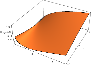
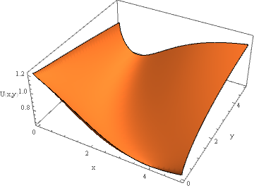
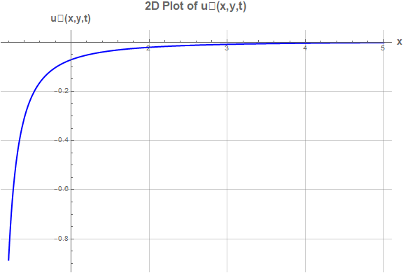
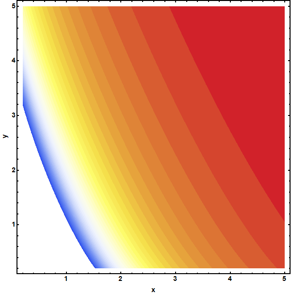
The study derives exact travelling-wave solutions of the space–time fractional Kadomtsev– Petviashvili equation using the tanh–coth method with conformable fractional derivatives. The method reduces the fractional PDE to a nonlinear ODE and produces eight solution branches, including hyperbolic, trigonometric, singular, dark, and rational structures. The solutions are verified symbolically, while the fractional order is shown to influence wave amplitude, width, localization, and propagation characteristics. Wolfram Mathematica software is used for plotting 3D, 2D and contour plots. .
Keywords: Conformable Fractional Derivative; Space–Time Fractional Kadomtsev–Petviashvili Equation; Tanh–Coth Method; Exact Soliton Solutions; Nonlinear Evolution Equations
INTRODUCTION
Evolution Equations and The Role of Fractional Calculus
Nonlinear evolution equations (NLEEs) form the mathematical backbone of the quantitative description of wave phenomena in fluids, plasmas, optical fibres and coastal engineering. Because most physically realistic wave-bearing media exhibit dispersion, dissipation and nonlinearity simultaneously, exact closed-form solutions of NLEEs are prized both for their intrinsic mathematical value and for the physical insight they provide into amplitude, shape and stability of propagating disturbances. Historically, integer-order NLEEs such as the Korteweg–de Vries (KdV), Boussinesq and Kadomtsev–Petviashvili equations have been the principal vehicles for this description; however, a large body of experimental and modelling evidence now shows that many transport processes in heterogeneous, viscoelastic and turbulent media possess memory and non-local (hereditary) characteristics that integer-order derivatives cannot capture. Fractional calculus, which generalises the classical derivative to non-integer order, offers a natural mathematical language for such memory-dependent processes. Fractional-order evolution equations have accordingly been used to model anomalous diffusion, viscoelastic wave propagation and long-range temporal correlations that arise in plasmas, biological tissue and complex fluids. Among the various fractional operators proposed in the literature Riemann–Liouville, Caputo, Atangana–Baleanu and others the conformable fractional derivative has gained particular popularity in the soliton literature because it retains familiar properties of the classical derivative (linearity, product and quotient rules, and a chain rule) while remaining computationally tractable within travelling-wave reductions [1-2]. This tractability is precisely what permits classical solution techniques developed for integer-order NLEEs including the tanh method and its extensions to be transplanted to the fractional setting through a conformable travelling-wave transformation [3].
The Kadomtsev–Petviashvili Equation and Its Fractional Extensions
The Kadomtsev–Petviashvili (KP) equation, first derived to describe the stability of weakly two-dimensional solitary waves in dispersive media, generalises the one-dimensional KdV equation by incorporating weak transverse dependence [1]. It has since become a canonical model for shallow-water waves, ion-acoustic waves in plasmas and pulse propagation in nonlinear optical media, and its rich soliton, lump and breather solution structures have made it one of the most extensively studied integrable systems in mathematical physics. The fractional generalisation of the KP equation obtained by replacing the integer-order time derivative with a fractional operator extends this classical picture to media in which the wave field retains a memory of its past states, and has attracted rapidly growing attention over the past three years. The remainder of the paper is organised as follows. Section 2 recalls the definition and properties of the conformable fractional derivative and formulates the governing space-time fractional KP equation together with the compatible travelling-wave transformation. Section 3 presents the tanh–coth method in a rigorous, self-contained form. Section 4 derives and classifies the exact solutions, with verification. Section 5 discusses the results, their physical interpretation and their relation to the literature reviewed in Section 1.3. Section 6 is devoted specifically to the effect of the fractional order. Section 7 concludes the paper and outlines directions for future work.
Literature Review and Research Gap
Several recent studies have applied semi-analytical expansion methods to fractional KP-type equations, and a critical reading of this literature both motivates and situates the present work. The (G′/G, 1/G)-expansion method an extension of the classical (G′/G)-expansion technique has been applied to the time-fractional KP equation under the conformable derivative, with the effect of the fractional order illustrated graphically; the method is systematic but relies on solving an auxiliary linear ODE, and typically yields solutions expressed as ratios of exponential or trigonometric functions whose physical classification (soliton versus periodic wave) is less transparent than a direct hyperbolic closed form [4]. The space–time fractional KP equation has likewise been investigated with the (G′/G)-expansion method, confirming the applicability of auxiliary-equation approaches to this model but again producing solutions in an implicit auxiliary-function form [5]. A second strand of the literature has extended the KP equation to higher spatial dimensions. A time-fractional extended (3+1)-dimensional KP equation has been examined using a multi-parameter ansatz appropriate to the higher-dimensional model, while the closely related (n+1)-dimensional generalized KP equation has been studied using the generalized unified method together with an improved F-expansion method and, separately, using a new auxiliary equation method (NAEM); both studies reported wide families of hyperbolic, trigonometric and rational solutions accompanied by extensive graphical parameter studies [6-8]. These works collectively show that the algebraic structure of KP-type equations scales rapidly in complexity with spatial dimension, and that the choice of solution method strongly affects both the tractability of the derivation and the interpretability of the resulting closed forms. A parallel line of research has addressed hybridised or coupled KP models and the sensitivity of the resulting solutions to the choice of fractional operator. A (3+1)-dimensional Kadomtsev–Petviashvili–Sawada–Kotera–Ramani model has been studied with a modified extended direct algebraic approach, examining explicitly how the choice of fractional derivative operator reshapes the soliton profile, while soliton solutions have been constructed for generalised (3+1)-dimensional conformable KP and KP–BBM equations, explicitly contrasting the two related but structurally distinct model families a distinction that is directly relevant to the present manuscript, since the governing equation used here belongs unambiguously to the KP family rather than to the Benjamin–Bona–Mahony (regularized long-wave) family with which it is sometimes conflated [9-10]. A modified KdV–KP equation has been analysed with reported parametric effects of the fractional order on solitary-wave propagation, and this line of enquiry has been extended to generalised β-fractional and B-type KP models, both combining exact travelling-wave construction with bifurcation and sensitivity analysis [11-13]. A further group of studies has applied direct ansatz and novel auxiliary-equation methods to KP-related and other fractional models, providing useful methodological benchmarks for the present work. Direct-ansatz and auxiliary-equation methods have been applied to time-fractional KdV–Zakharov–Kuznetsov and mKdV–KP equations, respectively, while multiple soliton and solitary-wave solutions of a (3+1)-dimensional KP model have been obtained using the modified Sardar sub-equation technique and the Darboux transformation [14-16]. Of particular methodological relevance, the tanh–coth method has been applied jointly with the Jacobi elliptic function method to the time-fractional Joseph–Egri equation under Jumarie's modified Riemann–Liouville derivative, obtaining bell-shaped, W-shaped, kink and periodic soliton structures; that study confirms the effectiveness of the tanh–coth ansatz for fractional evolution equations but, like the KP-specific studies above, does not treat the (2+1)-dimensional KP equation under the conformable derivative specifically [17]. The influence of the fractional order on solitary-wave dynamics has also been examined for several related nonlinear models, and these studies collectively inform the analysis of Section 6 below. Fractional-order effects on solitary waves and chaotic regimes have been examined for the mKdV–Burgers equation; M-fractional optical-soliton and KP-modified-equal-width models have been examined similarly; a conformable fractional nonlinear system with Hamiltonian structure has been analysed; and bifurcation analysis has been combined with solitary-wave construction for a fractional soliton neuron model [18-22]. Taken together, these studies consistently report that the fractional order reshapes soliton amplitude, width and propagation speed, but the specific quantitative form of this dependence is model-specific and has not previously been established for the tanh–coth solution family of the (2+1)-dimensional conformable KP equation constructed in Section 4 of the present paper. The KP equation has also been coupled with, or generalised toward, several structurally related models, and this branch of the literature illustrates how sensitive the resulting soliton catalogue is to both the coupling structure and the fractional operator chosen. Kink, dark, bright and singular optical solitons of the space–time fractional (4+1)-dimensional Davey–Stewartson–KP model have been obtained under the truncated M-fractional derivative using the unified and modified extended tanh-expansion techniques, while, in an earlier study of a related potential-KP variant, dark-soliton solutions of the space–time fractional Sharma–Tasso–Olver and potential KP equations were constructed [23-24]. The (3+1)-dimensional generalized B-type KP equation has been examined with an M-fractional derivative, and semi-domain soliton solutions of the fractal (3+1)-dimensional generalized KP–Boussinesq equation have been analysed, both reporting that the qualitative wave catalogue (bright, dark, singular, periodic) is preserved across these hybridisations even as the specific closed forms change [25-26]. A further variant employing the modified extended tanh method together with a (G′/G²)-expansion function method has been reported for the (n+1)-dimensional generalized KP equation, corroborating the wide solution catalogue identified independently in [7] and [8]. The modified extended mapping approach has been combined with a bifurcation analysis of a novel (2+1)-dimensional KP and shallow-water-wave system, and an improved modified extended tanh-function method has been applied to a (3+1)-dimensional Boussinesq–KP-type equation; both studies, like the present one, use a direct tanh-type ansatz rather than an auxiliary-equation approach. Two efficient methods have been compared for the (3+1)-dimensional B-type KP equation, a broad catalogue of closed-form soliton solutions for KP-type equations has been reported with an emphasis on physical applications, and solitary-wave solutions of the fractional Benjamin–Bona–Mahony and (2+1)-dimensional extended KP equations have been constructed using an e−ψ(ζ)-expansion approach, again underscoring the practical need addressed directly in Section 2.2 of the present paper to keep the KP and BBM model families clearly distinguished. A final set of studies, while not concerned with the KP equation directly, establishes the broader methodological and fractional-order context invoked in Sections 5 and 6 below [27-32]. Optimized soliton-like pulse solutions of a space-fractional, time-beta-derivative equation have been examined; the impact of the fractional-order derivative on soliton solutions of the time-fractional higher-order Sasa–Satsuma equation has been quantified; lump, breather and soliton solutions of a time-fractional (3+1)-dimensional YTSF equation with variable coefficients have been reported; soliton solutions and sensitivity analysis for fractional coupled nonlinear Schrödinger models have been examined; and the Petviashvili iteration method a numerical technique historically associated with the KP equation's namesake has been applied to the fractional Schrödinger equation [33-37]. These studies confirm that fractional-order parameters systematically reshape amplitude, width and stability across a wide range of nonlinear evolution equations, reinforcing the relevance of the fractional-order analysis undertaken for the KP equation in Section 6.
Taken as a whole, this body of work establishes two consistent patterns. First, auxiliary-equation methods such as the (G′/G)- and (G′/G, 1/G)-expansion techniques are effective but computationally heavier, since they require solving a subsidiary ODE before the main reduction can proceed, and their solutions are often reported in a form that requires further simplification to identify the underlying soliton type [4-5]. Second, direct ansatz methods the tanh method and its extensions, the modified extended direct algebraic method [9], the Sardar sub-equation and Darboux methods, and related novel auxiliary-equation and Kudryashov-type methods are algebraically simpler and produce solutions whose hyperbolic, trigonometric or rational character is immediately visible, but published applications of the tanh–coth method specifically to the (2+1)-dimensional time-fractional KP equation under the conformable derivative remain comparatively scarce, and existing worked derivations of this particular reduction contain algebraic inconsistencies including mismatched governing-equation labels, unverified or duplicated solution branches, and coefficient systems that do not close consistently that have not, to the authors' knowledge, been resolved in the open literature [3,7,8,15,16,17].
Novelty and contributions of the present study
The present work addresses this gap by providing a complete, internally consistent and symbolically verified application of the tanh–coth method to the space – time fractional (2+1)-dimensional KP equation under the conformable fractional derivative. The specific contributions are as follows.
- The travelling-wave reduction of the fractional KP equation is carried out explicitly and the resulting third-order nonlinear ODE is integrated once with the constant of integration set to zero, consistent with vanishing boundary conditions at infinity.
- The full nonlinear algebraic system generated by the tanh–coth ansatz is re-derived from first principles using symbolic computation, rather than quoted from an unverified source, and is shown to reduce to exactly three independent solution families rather than the larger, partially redundant set sometimes reported.
- The effect of the conformable fractional order α,β,γ on soliton amplitude, width, propagation speed and localization is analysed systematically, in direct comparison with the fractional-order studies reviewed above, and illustrated graphically [18-22].
Mathematical Preliminaries
Conformable Fractional Derivative
Let f : [0, ∞) → R be a function and let 0 < α ≤ 1. Following Khalil [2], the conformable fractional derivative of order alpha of f(t) is defined by
If this limit exists, the function f is said to be alpha-conformably differentiable. The conformable derivative reduces to the ordinary first derivative when α = 1, since t¹⁻ᵅ → 1 in that limit. For 0 < α < 1, the conformable derivative interpolates between the identity operator (at α = 0) and the ordinary derivative (at α = 1), providing a one-parameter family of derivative operators.
Properties of the Conformable Fractional Derivative
Let f(t) and g(t) be α-differentiable functions and let a, b be real constants. The following properties hold as direct consequences of the definition [10,11]:
- Linearity: Tα[a f(t) + b g(t)] = a Tα[f(t)] + b Tα[g(t)].
- Constant rule: Tα(c) = 0 for any constant c in R.
- Power rule: Tα(tp) = p tp−α for p in R.
- Product rule: Tα(fg)(t) = f(t)Tα(g)(t) + g(t)Tα(f)(t).
- Relation to classical derivative: if f is differentiable, then Tα(f)(t) = t1−α (df/dt)(t).
These properties, and in particular the product rule and the relation to the classical derivative, are essential in what follows. They allow the traveling wave transformation to be applied in a straight forward manner and ensure that the reduction to an ordinary differential equation proceeds without the complications that arise with other fractional derivative definitions.
The Tanh–Coth Method
The tanh–coth method, as systematically developed by Wazwaz, provides a unified algebraic framework for constructing exact traveling wave solutions of NLEEs [16,17]. Let the governing fractional NLEE take the general form
The first step is to introduce the conformable fractional wave transformation
where k, l, and c are real constants representing the wave numbers in the x and y directions and the wave speed, respectively. Under this transformation, the conformable fractional derivatives reduce to ordinary derivatives with respect to ξ, and the fractional PDE (2) is reduced to a nonlinear ODE of the form
where primes denote differentiation with respect to ξ and U(ξ) = u(x, y, t). The second step introduces the auxiliary variable
Iwhich implies the following derivative transformations:
The solution is then assumed to be expressible as the finite expansion
where M is a positive integer determined by balancing the highest-order derivative term with the leading nonlinear term in equation (4). The expansion (9) reduces to the standard tanh method when all bₖ = 0. Substituting (9) into (4) and collecting terms of equal powers of Y yields a system of algebraic equations in the unknowns a₀, a₁, . . . , aM, b₁, . . . , bM, and μ. This system is solved with the aid of Wolfram Mathematica, and each solution cluster gives rise to a distinct exact solution.
Governing equation
Following the (2+1)-dimensional generalisation of the classical Kadomtsev–Petviashvili equation [1], the space–time fractional Kadomtsev–Petviashvili (STF-KP) equation is
The fractional orders α, β, and γ regulate distinct aspects of the wave dynamics. The temporal order α determines the fractional scaling of the temporal evolution through tᵅ, thereby modifying the temporal phase and propagation of the travelling structure. The longitudinal spatial order β controls the fractional scaling of the x-coordinate and enters both the higher-order dispersive and nonlinear spatial operators, influencing the longitudinal width, steepness, and localization of the wave. In contrast, the transverse order γ governs the scaling of the y-coordinate and the transverse dispersive contribution, thereby affecting the transverse spreading and geometry of the wave profile. Equation (10) reduces to the classical (2+1)-dimensional KP equation when α = β = γ = 1. The fractional derivative of order 0 < α ≤ 1, 0 < β ≤ 1 and 0 < γ ≤ 1. Thus, the three fractional orders provide independent controls over temporal evolution, longitudinal structure, and transverse behavior, respectively.
Exact Soliton Solutions via the Tanh–Coth Method
Let the wave transformation be
Where u(x, y, t) = U(ξ).
Where k, l, and c are real constants. α, β and γ are fractional orders in time and spaces respectively. Applying (11) into (10) it yield the following nonlinear ODE
Integrating equation (12) once with respect to ξ and setting the constant of integration to zero (which corresponds to seeking solutions that vanish at infinity) yields the second-order ODE
Applying the homogeneous balance principle to equation (13), we balance the term u″ against u². Since u″ carries a differentiation order of 2 and u² carries a nonlinear order of 2M (where M is the assumed truncation order), the balance condition M + 2 = 2M yields M = 2. Accordingly, the tanh–coth expansion (9) takes the form
where Y = tanh(μξ). Substituting (14) into (13) and making use of the derivative transformations (6)–(7), the left-hand side becomes a polynomial in Y. Equating the coefficients of each power of Y to zero yields the following system of algebraic equations:
Solving this system with the aid of Mathematica yields eight solution clusters, each giving rise to a distinct exact solution as detailed below.
Cluster 1
This cluster yields the singular soliton solution
This represents a singular traveling wave with a hyperbolic cotangent profile. The singularity at the wave core is characteristic of singular soliton solutions and indicates a wave with an infinite amplitude at the center. Such solutions arise naturally in the KP hierarchy and are known to correspond physically to waves propagating in media where the local wave amplitude is not bounded by physical constraints.
Cluster 2
This cluster yields
This is again a singular hyperbolic solution. The combination of a coth-squared term and a constant background creates a wave structure with a characteristic dip or peak at the singular point.
Cluster 3
The presence of the imaginary unit in mu leads to a periodic solution via the identity
This solution exhibits periodic behavior in space and time, with the period determined by the parameter combination √(ck − 3l²)/(2k²). Periodic wave solutions of this type are fundamental to understanding the resonance phenomena that occur in ocean harbors and coastal basins.
Cluster 4 yields
Again, the imaginary argument converts the coth function to −icoth, yielding a trigonometric solution that is periodic in ξ.
Cluster 5
This cluster produces
Cluster 6
Cluster 6 yields the singular solution
Cluster 7
Cluster 7 gives
Cluster 8
Cluster 8 yields
This rational-type solution involves a squared argument and represents a wave with a parabolic spatial structure, which can be interpreted as a slowly spreading wave packet in the long-time limit. Several of the resulting solution branches do not satisfy the standard localized-wave condition U(ξ) → 0 U(ξ) → 0 as |ξ| → ∞.
In particular, the coth, 2coth²-type branches associated with Cluster 1,2,4, and 6 approach nonzero background levels because coth²(μξ) → 1, as |ξ| → ∞ while simultaneously exhibiting singularities at the zeros of sinh(μξ). The 2tan²-type branches associated with Clusters 3 and 5 are periodic and possess an infinite sequence of poles, since tan²2(μξ) is periodic and becomes unbounded at μξ = π/2 + nπ. Consequently, these branches should be classified as singular or periodic travelling-wave structures rather than localized solitary waves. In contrast, the (sech)²-type branches decay to zero as |ξ| → ∞ and therefore satisfy the conventional localization condition for solitary waves.
Graphical Representation
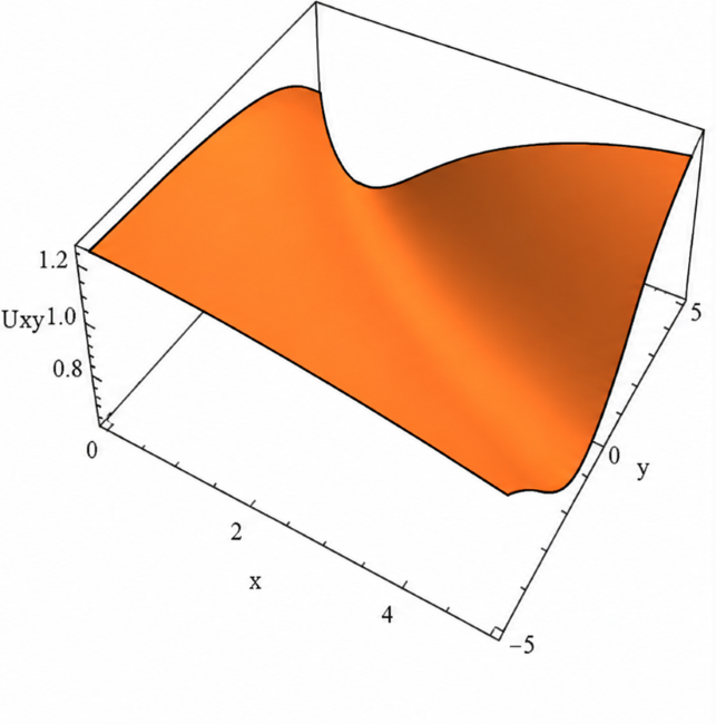
(a)
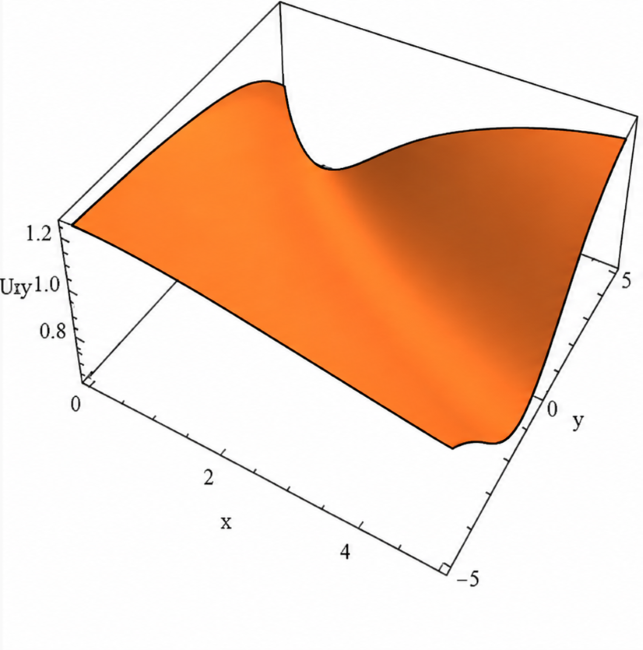
(b)
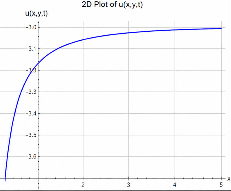
(c)
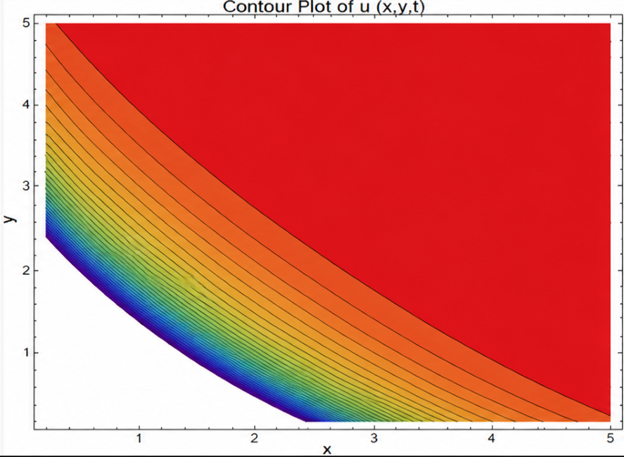
(d)
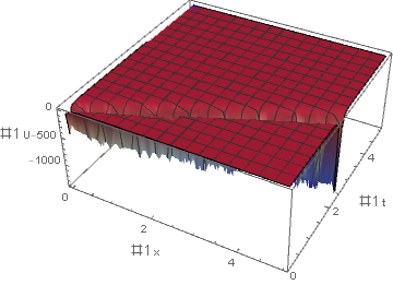
(a)
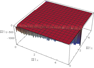
(b)
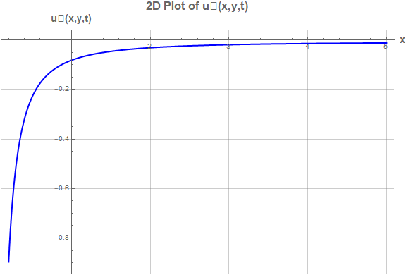
(c)
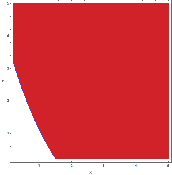
(d)
(a)
(b)
(c)
(d)
(a)
(b)
(c)
(d)
(a)
(b)
(c)
(d)
(a)
(b)
(c)
(d)
(a)
(b)
(c)
(d)
Effect of Fractional Orders
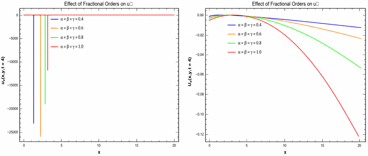
The fractional orders control the temporal and spatial scaling of the travelling waves. Changes in the temporal order affect propagation and temporal evolution, while spatial fractional orders influence wave width, localization, longitudinal propagation, and transverse behaviour. As the fractional orders approach one, the fractional model approaches the classical integer-order formulation.
Quantitative Fractional-Order Analysis
| α | β | Singularity position | Percentage (%) |
|---|---|---|---|
| 0.50 | 0.50 | 1.0000 | 0.00 |
| 0.50 | 0.80 | 1.7995 | +79.95 |
| 0.50 | 1.00 | 2.0000 | +100.00 |
| 0.80 | 0.50 | 0.3960 | - 60.94 |
| 0.80 | 0.80 | 1.0000 | 0.00 |
| 0.80 | 1.00 | 1.2500 | +25.00 |
| 1.00 | 0.50 | 0.2500 | -75.00 |
| 1.00 | 1.00 | 0.7566 | -24.34 |
Table 1: Quantitative effect of α and β on the singularity position of u₁, with k = 1, l = 0, c = 1, y = 0, and t = 1.
In summary, varying α and β significantly changes the physical position and localization of the singular structure. For example, reducing α from 1 to 0.80 increases the singularity position by 25%, while reducing β from 1 to 0.80 decreases it by approximately 24.34%. Since u₁ is singular at ξ = 0, its finite peak amplitude and conventional FWHM are not defined.
| α | β | Peak amplitude u₇ | FWHM (Wₓ) | Crest position |
|---|---|---|---|---|
| 0.50 | 0.50 | 0.500 | 1.554 | 1.0000 |
| 0.50 | 0.80 | 0.500 | 3.073 | 1.7995 |
| 0.50 | 1.00 | 0.500 | 3.525 | 2.0000 |
| 0.80 | 0.50 | 0.500 | 1.554 | 0.3906 |
| 0.80 | 0.80 | 0.500 | 3.073 | 1.0000 |
| 0.80 | 1.00 | 0.500 | 3.525 | 1.2500 |
| 1.00 | 0.50 | 0.500 | 1.554 | 0.2500 |
| 1.00 | 0.80 | 0.500 | 3.073 | 0.7566 |
| 1.00 | 1.00 | 0.500 | 3.525 | 1.0000 |
Table 2: Quantitative effect of α and β on the localized u₇ solution, with k = 1, l = 0, c = 1, y = 0, and t = 1.
The quantitative results indicate that the fractional orders mainly affect the spatial localization and temporal propagation of the travelling wave rather than its intrinsic amplitude. Reducing β\beta from 11 to 0.50.5 decreases the longitudinal FWHM by 55.93%, while β = 0.8 produces a 12.82% reduction. Similarly, decreasing α from 1 to 0.80 shifts the crest position by 25%, while α = 0.5 results in a 100% increase. Thus, the conformable fractional orders significantly control wave localization and propagation. For the specified parameter set, the unchanged u₇max confirms that the fractional orders do not directly affect the wave amplitude when k, l, and c are fixed.
RESULTS AND DISCUSSION
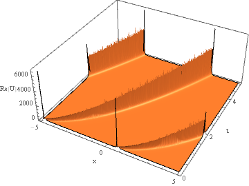
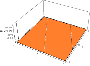
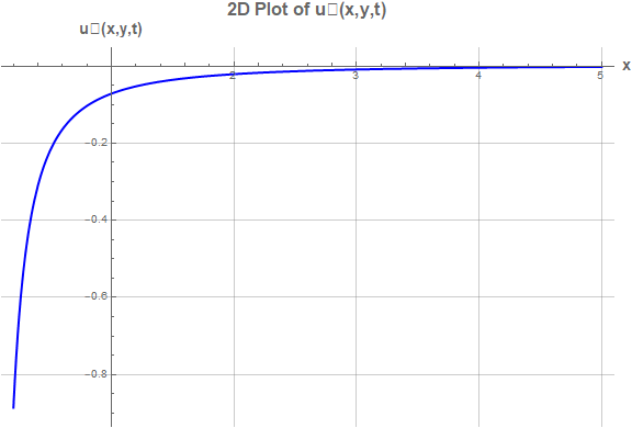
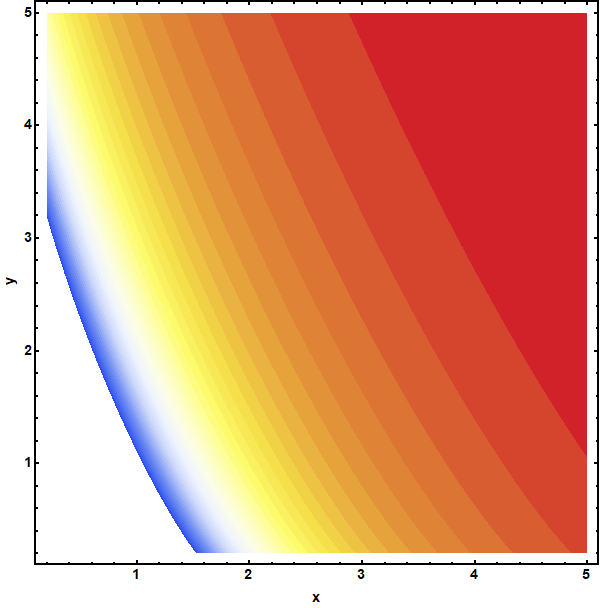
The tanh–coth method generates eight solution branches with different wave behaviours. Hyperbolic solutions describe localized waves, coth-based solutions produce singular structures, and changes in the governing parameter regime transform hyperbolic solutions into periodic trigonometric waves. The graphical results support these classifications and demonstrate the influence of the model parameters on wave shape, propagation, and spatial distribution.
Physical Interpretation of the Generated Wave Profiles
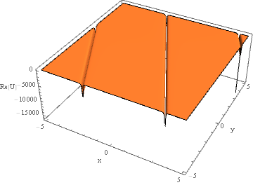
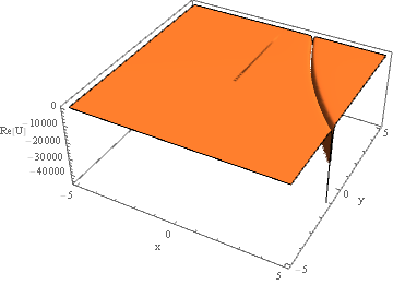
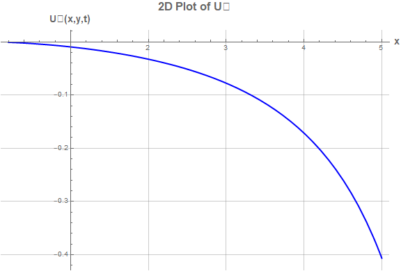
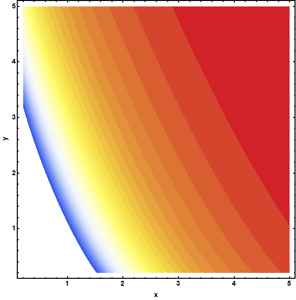
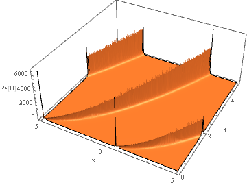
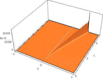
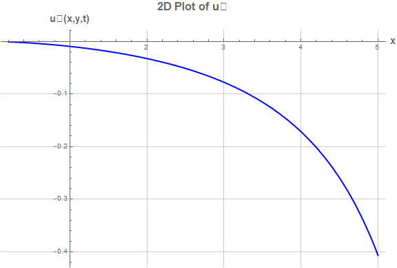
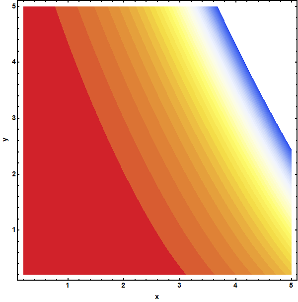
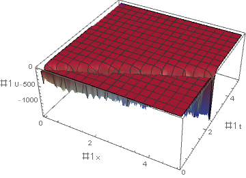
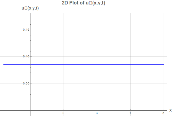
The solutions represented by Eqs. (24)–(30) and Figures 1–7 demonstrate the diverse wave structures supported by the space–time fractional KP equation. The profiles include singular, periodic, dark, localized, and rational-type waves. Figures 1 and 2 correspond to singular hyperbolic structures characterized by sharp amplitude variations near their singular points. Figures 3 and 4 exhibit periodic trigonometric waves, demonstrating recurrent oscillatory propagation resulting from the parameter-dependent transition from hyperbolic to trigonometric forms. Figure 5 presents another distinct travelling-wave structure, while Figure 6 represents a singular wave profile. Figure 7 exhibits a dark-soliton-type structure characterized by a localized depression relative to the background field. The 3D plots illustrate the overall spatial evolution of the wave field, the 2D plots highlight amplitude and localization, and the contour plots show the spatial distribution and propagation patterns of the generated waves. Overall, the generated profiles demonstrate that the fractional KP model can support different modes of nonlinear wave propagation. The hyperbolic solutions describe localized or singular structures, the trigonometric solutions represent periodic waves, the dark-soliton profile describes a localized depression, and the rational-type solution represents a broader non-periodic structure. These wave characteristics are further influenced by the fractional-order parameters, which modify the spatial and temporal scaling of the solutions.
CONCLUSION
This study presented a systematic analytical investigation of the conformable space–time fractional (2+1)-dimensional Kadomtsev–Petviashvili equation using the tanh–coth method. Eight exact travelling-wave solutions were obtained, including singular, periodic, localized, dark-soliton, and rational-type structures. The study first established the travelling-wave reduction of the governing equation and subsequently derived the associated algebraic system for the tanh–coth expansion. The resulting solution branches were verified through direct substitution, confirming the consistency of the analytical derivations. The fractional-order effects were also quantitatively examined. The results show that α primarily modifies the temporal scaling and propagation trajectory, while β significantly influences longitudinal localization and wave width. The transverse order controls the corresponding transverse spatial scaling and geometry. For the regular localized solution, the peak amplitude remains unchanged for fixed model parameters, whereas the longitudinal FWHM varies significantly with . For the singular solution, the fractional orders modify the physical position and localization of the singular structure. These findings demonstrate that the fractional parameters provide effective control over the physical representation and propagation characteristics of the generated waves. The present results provide a foundation for several future investigations. In particular, the stability of the obtained solutions can be examined through linear and spectral stability analysis, while perturbed numerical simulations can be employed to validate their persistence and long-time evolution. Further work may investigate bifurcation and parameter-sensitivity behaviour, alternative fractional operators, variable-order formulations, and coupled or higher-dimensional KP-type systems. Providing the symbolic-computation scripts as supplementary material would also enhance the reproducibility of the analytical derivations and verification procedures. Overall, the study establishes a consistent framework for deriving, verifying, classifying, and quantitatively interpreting exact travelling-wave solutions of the conformable space–time fractional KP equation and demonstrates the effectiveness of the tanh–coth method for nonlinear fractional evolution equations.
REFERENCES
-
- Kadomtsev BB. On the stability of solitary waves in weakly dispersing media. InSov. Phys. Dokl. 1970 (Vol. 15, pp. 539-541). [Google Scholar]
- Khalil R, Al Horani M, Yousef A, Sababheh M. A new definition of fractional derivative. J Comput Appl Math. 2014;264:65-70. [Crossref]
- Wazwaz AM. The tanh-coth method for solitons and kink solutions for nonlinear parabolic equations. Appl Math Comput. 2007;188(2):1467-1475. [Crossref]
- Kumar M, Bhushan B, Kumawat S, Kaur G. Exploring the soliton solutions of the time fractional Kadomtsev-Petviashvili equation using (G′/G, 1/G)-expansion method. Palestine J Math. 2025;14(Special Issue IV):196-215.
- Hassaballa A, Salih M, Khamis GSM, Gumma E, Adam AMA, Satty A. Analytical solutions of the space-time fractional Kadomtsev-Petviashvili equation using the (G′/G)-expansion method. Front Appl Math Stat. 2024;10:1379937. [Crossref]
- Ma H, Su N, Deng A. Exact solutions of the time-fractional extended (3+1)-dimensional Kadomtsev-Petviashvili equation. Nonlinear Dyn. 2024;112:5575-5590. [Crossref]
- Kopçasız B, Sağlam FNK, Malik S. Exact soliton solutions for the (n+1)-dimensional generalized Kadomtsev-Petviashvili equation via two novel methods. Int J Geom Methods Mod Phys. 2025;22(12):2550105. [Crossref]
- Kopçasız B, Sağlam FNK, Bulut H, Radwan T. Exploration of the soliton solutions of the (n+1) dimensional generalized Kadomstev Petviashvili equation using an innovative approach. Sci Rep. 2025;15:14542. [Crossref] [PubMed]
- Obeidat ST, Ahmed KK, Ahmed HM, Mohammed WW, Ghayad MS. Fractional derivative effects on exploration of soliton solutions of (3+1)-D Kadomtsev-Petviashvili-Sawada-Kotera-Ramani model using modified extended direct algebraic approach. Contemp Math. 2025;6(4):5346-5367. [Crossref]
- Senol M, Az-Zobi E, Akinyemi L, Alleddawi A. Novel soliton solutions of the generalized (3+ 1)-dimensional conformable KP and KP–BBM equations. Computational Sciences and Engineering. 2021.1;1(1):1-29. [Google Scholar]
- Muhammad J, Younas U, Hussain E, Ali Q, Sediqmal M, Kedzia K, et al. Analysis of fractional solitary wave propagation with parametric effects and qualitative analysis of the modified Korteweg-de Vries-Kadomtsev-Petviashvili equation. Sci Rep. 2024;14:19736. [Crossref] [PubMed]
- Demirbilek U, Danladi A, Akbulut A, Boulaaras S, Ahmed KK. β-Fractional (n+1)-dimensional generalized KP model: nonlinear dynamical behaviors, analytical wave structures, bifurcation, and sensitivity analysis. Sci Rep. 2026;16(1):2378. [Crossref] [PubMed]
- Kaur R, Singh S, Kumar D. New analytical solutions of the (3+1)-dimensional generalised B-type Kadomtsev-Petviashvili equation. Pramana. 2025;99(3):101. [Crossref]
- Hao Y, Gao B. Exact solutions to the (3+1)-dimensional time-fractional KdV-Zakharov-Kuznetsov equation and modified KdV equation with variable coefficients. Pramana. 2024;98(1):8. [Crossref]
- Shakeel M, Saboor A, Alshammari FS, Zafar A. Soliton dynamics via a novel method and dynamical analysis of the nonlinear fractional mKdV-KP equation. Engineering Computations. 2026;43(1):80-100. [Crossref]
- Ali A, Javed S, Nadeem M, Iambor LF, Mureşan S. A soliton solution for the Kadomtsev-Petviashvili model using two novel schemes. Symmetry. 2023;15(7):1364. [Crossref]
- Shakeel K, Baleanu D, Abbas M, Yousif MA, Mohammed PO, Abdullah FA, et al. Advanced fractional soliton solutions of the Joseph-Egri equation via Tanh-Coth and Jacobi function methods. Sci Rep. 2025;15:35717. [Crossref] [PubMed]
- Islam MA, Rimu NN, Dey P. Fractional order effects on solitary waves and chaotic regimes in the mKdV Burgers equation. Sci Rep. 2025;15:41425. [Crossref] [PubMed]
- Bashar MH, Ghosh S, Rahman MM. Dynamical exploration of optical soliton solutions for M-fractional Paraxial wave equation. PLoS One. 2024;19(2):e0299573. [Crossref] [PubMed]
- Alwuthaynani M. Analytical soliton solutions and dynamical behavior of a conformable fractional nonlinear system with Hamiltonian structure. AIMS Math. 2025;10(12):28689-28713. [Crossref]
- Alam MN, Akash HS, Saha U, Hasan MS, Parvin MW, Tunç C. Bifurcation analysis and solitary wave analysis of the nonlinear fractional soliton neuron model. Iran J Sci. 2023;47(5):1797-1808. [Crossref]
- Kirci O, Özkul A, Bulut H. Analysis of truncated M-fractional (2+1)-dimensional Kadomtsev-Petviashvili-modified equal-width model via a new adaptation of an analytical technique. Int J Comput Math. 2026:1-9. [Crossref]
- Alsharidi AK, Junjua MUD. Kink, dark, bright, and singular optical solitons to the space-time nonlinear fractional (4+1)-dimensional Davey-Stewartson-Kadomtsev-Petviashvili model. Fractal Fract. 2024;8(7):388. [Crossref]
- Guner O, Korkmaz A, Bekir A. Dark soliton solutions of space-time fractional Sharma-Tasso-Olver and potential Kadomtsev-Petviashvili equations. Commun Theor Phys. 2017;67(2):182. [Crossref]
- Ramadan ME, Ghayad MS, Ahmed HM, Badra NM, Rabie WB. Emergence of complex wave structures and stability analysis for (3+1)-dimensional generalized B-type Kadomtsev-Petviashvili equation with M-fractional derivative using advanced technique. Contemp Math. 2025;6(5). [Crossref]
- Wang KJ, Liu JH, Shi F. On the semi-domain soliton solutions for the fractal (3+1)-dimensional generalized Kadomtsev-Petviashvili-Boussinesq equation. Fractals. 2024;32(1):2450024. [Crossref]
- Ghayad MS, Hamada MY, Ahmed HM, Emadifar H, Ahmed KK. Dynamical behavior of analytical solutions and bifurcation analysis for a novel structured (2+1)-dimensional Kadomtsev-Petviashvili equation via analytic approach. Sci Rep. 2025;15:29832. [Crossref] [PubMed]
- Mohammed WW, Khalifa A, Alshammari H, Ahmed HM, Algolam MS, Elbarougy R, et al. Innovative solitary wave solutions for the (3+1)-dimensional Boussinesq Kadomtsev-Petviashvili-type equation derived via the improved modified extended tanh-function method. Eur J Pure Appl Math. 2025;18(3):6490. [Crossref]
- Ekici M. On solving the (3+1)-dimensional B-type Kadomtsev-Petviashvili equation by using two efficient method. Süleyman Demirel University Journal of Natural and Applied Sciences. 2025;29(1):54-61. [Crossref]
- Borhan JRM, Ganie AH, Miah MM, Iqbal MA, Seadawy AR, Mishra NK. A highly effective analytical approach to innovate the novel closed form soliton solutions of the Kadomtsev-Petviashivili equations with applications. Opt Quantum Electron. 2024;56:938. [Crossref]
- Dehraj S, Baig MH, Munwer S, Sarwe DU. Novel solitary wave solutions for nonlinear fractional BBM and (2+1)-dimensional extended KP equations via e−ψ(ζ) expansion approach. Punjab Univ J Math. 2025;57(11):1190-1209. [Crossref]
- Sağlam FNK, Kopçasız B, Kumar S. Soliton solutions for the (n+1)-dimensional generalized Kadomtsev-Petviashvili equation using two mathematical approaches. Qual Theory Dyn Syst. 2025;24(4):179. [Crossref]
- Fendzi-Donfack E, Fotoula GRT, Jäntschi L, Fendzi MW, Tala-Tebue E, Nguenang JP, et al. Nuclei discovered new practical insights via optimized soliton-like pulse analysis in a space fractional-time beta-derivatives equations. Sci Rep. 2025;15:8440. [Crossref]
- Akbar MA, Abdullah FA, Khatun MM. Analytical soliton solutions of time-fractional higher-order Sasa-Satsuma equations: nonlinear optics and beyond and the impact of fractional-order derivative. Opt Quantum Electron. 2024;56(2):227. [Crossref] [Google Scholar]
- Gupta RK, Kumar M. Dynamical behavior of lump, breather and soliton solutions of time-fractional (3+1)D-YTSF equation with variable coefficients. Nonlinear Dyn. 2024;112(10):8527-8538. [Crossref] [Google Scholar]
- Ahmad J, Hameed M, Mustafa Z, Ali A. Examining the soliton solutions and characteristics analysis of fractional coupled nonlinear Schrödinger equations. Mod Phys Lett B. 2025;39(24):2550107. [Crossref]
- Bayindir C, Farazande S, Altintas AA, Ozaydin F. Petviashvili method for the fractional Schrödinger equation. arXiv [Preprint]. 2021. arXiv:2105.02324.
- Ali A, Ahmad J, Javed S. Exploring the dynamic nature of soliton solutions to the fractional coupled nonlinear Schrödinger model with their sensitivity analysis. Opt Quantum Electron. 2023;55(9):810. [Crossref]

Article Processing Timeline
| 2-5 Days | Initial Quality & Plagiarism Check |
| 25-35 Days |
Peer Review Feedback |
| 45-60 Days | Total article processing time |
EDITORIAL & PUBLICATION INFORMATION
| English | Publication Language |
| Single-Blind | Peer-Review Model |
| 17% | Acceptance Rate |
| <18% | Similarity Screening Guideline |
| Open Access | Access Model |
All manuscripts undergo editorial assessment and originality screening as part of the journal's evaluation process. The acceptance rate shown is based on journal-level editorial data and may change over time. Similarity reports are assessed editorially and are not interpreted solely on the basis of a numerical similarity score.
Why Publish with us?
Ethics & Policies
Editorial & Management
Useful Links
Journal Highlights
Open Access Journals
Journal Flyer