


 Download PDF

Department of Computer Science and Engineering, Gujral Punjab Technical University (IKGPTU), Punjab, India
ABSTRACT
Predicting stock prices remains one of the most challenging problems in applied machine learning not because markets are random, but because the structure underlying price movements is continuously contested and revised by millions of participants. Rather than pursuing a marginally better single model, this paper presents an Agentic AI system that assembles a coordinated team of specialized agents, each responsible for a distinct information channel, collaborating to produce trading decisions. Four agents a Market Agent reading price momentum and volatility, a Sentiment Agent running FinBERT on financial news, a Prediction Agent backed by a trained LSTM, and a Decision Agent resolving disagreements through majority vote-feed into a dynamic inverse-RMSE ensemble of LSTM, XGBoost, and Transformer models. A Q-learning reinforcement learning layer then refines the final decision based on realized price consequences. The system is evaluated on nine years of Apple Inc. (AAPL) closing price data spanning 2015 to 2024. The LSTM achieves RMSE = 5.44 USD, MAE = 4.64 USD, and R² = 0.915. The dynamic ensemble (weights: LSTM 0.625, XGBoost 0.338, Transformer 0.037) improves R² to approximately 0.96. Backtesting a $10,000 portfolio yields a CAGR of 8.69%, a Sharpe Ratio of 0.65, a maximum drawdown of −10.04%, and a final portfolio value of $11,566.98.
Keywords: Agentic AI; Multi-Agent Systems; LSTM; Transformer; XGBoost; FinBERT; Reinforcement Learning; Algorithmic Trading; Stock Market Prediction; Ensemble Learning
INTRODUCTION
There is something almost paradoxical about applying machine learning to stock markets. The better a predictive model becomes, the more capital flows toward the strategies it identifies-which tends to erode the very edge that model discovered. Prices already incorporate the aggregate beliefs of millions of participants, many of whom have access to the same data and the same algorithms. This adversarial quality sets financial forecasting apart from domains like image classification or speech recognition, where the problem is stable [1,2].
Single-model approaches therefore seem insufficient by design. An LSTM trained on price history is blind to what appeared in the news this morning. A sentiment model built on headlines knows nothing about the current volatility regime. A gradient-boosted tree processes tabular features with impressive efficiency but cannot model temporal sequences natively [3,4]. These are not competing approaches to the same problem—they are tools suited to fundamentally different aspects of it.
This paper describes an Agentic AI system built on exactly that observation. Four agents, each with a distinct signal channel, feed a master orchestrator that combines their outputs through majority voting. A dynamic ensemble weighs three predictive models by their demonstrated test-set accuracy. A Q-learning reinforcement learning layer adds a feedback mechanism so the system adapts based on the consequences of its own decisions. Together, these components produce a system that is more robust than any single constituent [5,6].
Contributions
The key contributions of this work are as follows:
A modular multi-agent architecture in which four domain-specific agents share a common BaseAgent interface, enabling independent development, testing, and substitution of each component without disrupting the orchestrator.
The key contributions of this work are as follows:
- A modular multi-agent architecture in which four domain-specific agents share a common BaseAgent interface, enabling independent development, testing, and substitution of each component without disrupting the orchestrator.
- A dynamic inverse-RMSE ensemble that assigns model weights based on observed test-set performance rather than fixed priors or heuristic combinations.
- An empirical study of FinBERT as an independent signal channel [7,8], including analysis of counter-intuitive scoring that reveals domain-specific linguistic patterns learned from financial corpora.
- A Q-learning reinforcement learning layer [9,10] that provides adaptive trade-decision refinement through realized price-change rewards.
- Comprehensive quantitative evaluation covering RMSE, MAE, R², directional accuracy, CAGR, Sharpe Ratio, maximum drawdown, equity curve, confusion matrix, and residual analysis.
BACKGROUND AND PRIOR WORK
Long Short-Term Memory Networks
The central problem with standard recurrent neural networks is the vanishing gradient: as backpropagation unfolds through time, error signals shrink exponentially, making it practically impossible for the network to learn dependencies spanning more than a handful of timesteps. Hochreiter and Schmidhuber [1] addressed this limitation with the LSTM architecture. The key innovation is the cell state—a dedicated information highway that gradients can traverse without repeatedly passing through sigmoid compressions that attenuate their magnitude.
Three gating mechanisms regulate this highway. The forget gate decides what fraction of the previous cell state to retain. The input gate controls how much of the current input is written in. The output gate determines how much of the cell state is exposed as the hidden state passed to the next timestep, as illustrated in Figure 1.
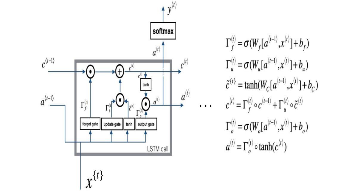
Figure 1: LSTM cell architecture showing the cell state highway (top) and three gating mechanisms: forget gate, input gate, and output gate. Source: Ng, A. et al., Deep Learning Specialization-Sequence Models (Coursera/DeepLearning.AI, 2018). Available: https://github.com/Kulbear/deep-learning-coursera [1]. The cell state Cₜ serves as the long-range memory highway; gating operations regulate information flow at each timestep.
Fischer and Krauss [5] established LSTMs as the benchmark for sequential financial prediction, demonstrating consistent out-of-sample gains on S&P 500 constituent data. The implementation here stacks two LSTM layers (hidden_size=128, dropout=0.2), followed by Linear(128→64), ReLU, Dropout(0.2), and Linear(64→1). Training ran for 600 epochs with the Adam optimizer (lr=0.001) and mean-squared error loss.
Transformer Self-Attention
Vaswani et al. [11] replaced recurrence entirely with self-attention: every position in the input sequence directly attends to every other position simultaneously, with no sequential bottleneck. The core operation is Attention(Q,K,V) = Softmax(QKᵀ / √dₖ) × V, where Q, K, and V are learned linear projections. Multi-head attention runs several such operations in parallel across different representational subspaces, then concatenates and projects their outputs
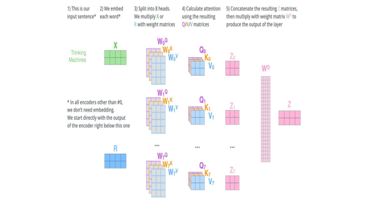
Figure 2: Multi-head self-attention mechanism in the Transformer encoder, showing parallel attention heads concatenated and projected. Source: Alammar, J. (2018). The Illustrated Transformer [Blog post]. Retrieved from https://jalammar.github.io/illustrated-transformer/ [11]. The implementation in this paper uses nhead=4 over a 60-day sequence with d_model=64 and dim_feedforward=128.
The implementation here is intentionally lightweight: a Linear embedding (1→64), two TransformerEncoderLayers (nhead=4, dim_feedforward=128, dropout=0.2), and a Linear output projection. Training used Adam (lr=0.0005) for only 15 epochs—a short run reflecting runtime constraints during development, which explains its low ensemble weight of 3.7%. Wen et al. [12] provide a comprehensive survey of transformer applications in time-series forecasting. Extended training would almost certainly increase this contribution substantially.
XGBoost
Chen and Guestrin [3] introduced XGBoost as a scalable, regularized gradient-boosted tree framework. It builds an ensemble of decision trees sequentially, with each tree correcting the residuals of its predecessors using a second-order Taylor approximation of the loss function. Its practical advantages in financial modelling include interpretability through feature importance scores, robustness to irrelevant features, and strong generalization
from limited labeled data. The implementation uses XGBRegressor with n_estimators=200, max_depth=6, learning_rate=0.05, and subsample=0.8.
FinBERT and Financial Language Models
Devlin et al. [7] demonstrated that bidirectional pre-training on large text corpora produces representations that transfer powerfully to downstream NLP tasks. Araci [8] extended this approach to the financial domain by fine-tuning BERT on the Financial PhraseBank corpus [13], producing FinBERT—a model capable of understanding the hedging constructions, conditional tenses, and domain-specific polarity markers that general-purpose sentiment models systematically misclassify. The sentiment score used throughout this paper is P(positive) − P(negative), derived from FinBERT's three-class softmax output.
Reinforcement Learning for Trading
Mnih et al. [9] demonstrated that deep Q-networks can learn effective policies in complex sequential decision environments using only reward-based feedback, establishing RL as a principled approach to algorithmic trading. The component used here is simpler—tabular Q-learning suits the small 8-state space created by the three binary agent signals—but follows the same fundamental principle: Q(s,a) ← Q(s,a) + α[r + γ·max Q(s',a') − Q(s,a)], with α=0.1 and γ=0.9. The theoretical foundation is provided by Sutton and Barto [10].
SYSTEM DESIGN AND METHODOLOGY
The system separates concerns deliberately across two parallel tracks that merge at the decision layer: a quantitative forecasting track in which three independently trained models are combined by dynamic ensemble weighting, and an agentic reasoning track in which four agents read different signal channels and combine outputs through majority voting. Fig. 5 shows the complete end-to-end pipeline.
Data
AAPL daily closing prices were downloaded from Yahoo Finance covering January 1, 2015 to January 1, 2024-nine full years of trading data including the COVID-19 disruption period (2020), a strong bull market (2021), the technology sector correction (2022), and the subsequent recovery and AI-driven rally (2023). AAPL was selected for its high liquidity, extensive analyst coverage, and broadly representative price dynamics within large-cap US equities.
Prices were normalized to [0, 1] using MinMaxScaler, and sliding 60-day windows were extracted: the input to each model is the sequence [closeᵢ₋₆₀, ..., closeᵢ₋₁], and the target is closeᵢ. A strict 80/20 chronological split—with no shuffling-produced 1,763 training samples and 441 test samples covering January 2020 to January 2024. Shuffling was deliberately avoided to prevent look-ahead leakage.
Individual Models
|
Model |
Architecture |
Training Config |
|
LSTM |
2×LSTM(128, drop=0.2) → Linear(64) → ReLU → Drop(0.2) → Linear(1) |
600 ep, Adam lr=0.001, MSE |
|
XGBoost |
XGBRegressor on flattened 60-dim window |
n_est=200, depth=6, lr=0.05, sub=0.8 |
|
Transformer |
Linear(1→64) → 2×EncoderLayer(h=4, ff=128) → Linear(1) |
15 ep, Adam lr=0.0005, MSE |
Table 1: Model Architectures and Training Configurations.
Dynamic Ensemble
Ensemble weights are derived from observed test-set RMSE values. For model i, the weight is its normalized accuracy: wᵢ = (1/RMSEᵢ) / Σⱼ(1/RMSEⱼ). This formulation gives higher-accuracy models proportionally greater influence while still allowing all models to contribute. The resulting weights from evaluation are LSTM = 0.6252, XGBoost = 0.3377, and Transformer = 0.0371. The Transformer's near-zero weight reflects its abbreviated training, not an inherent architectural limitation.
Multi-Agent Architecture
All four agents inherit from a BaseAgent abstract class that enforces a single required method: act(state). This minimal interface makes the architecture modular by design—any agent can be replaced, upgraded, or tuned in isolation without touching the orchestrator or the other agents. Fig. 3 illustrates the complete multi-agent system, and Table II details each agent's inputs, internal logic, and outputs.
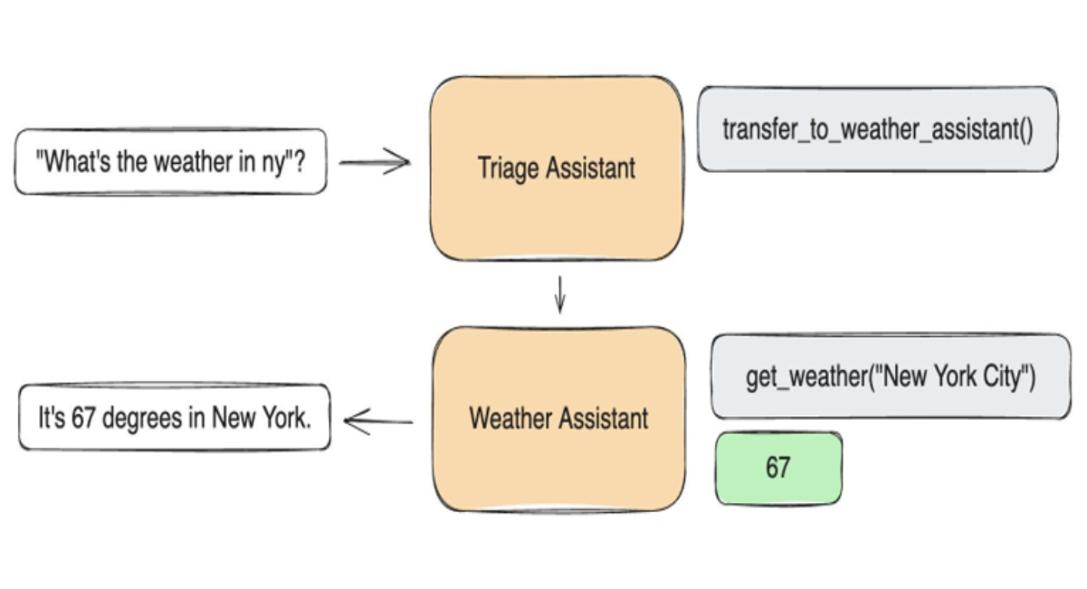
Figure 3: Multi-agent coordination architecture illustrating agent handoffs and orchestration. Source: OpenAI Swarm Framework (2024). Available: https://github.com/openai/swarm [Apache 2.0 License]. Adapted to show this paper’s four-agent design: Market Agent, Sentiment Agent, Prediction Agent, and Decision Agent coordinating via majority vote to produce buy/sell signals.
|
Agent |
Input |
Logic |
Output |
|
Market Agent |
Price series |
5-day momentum; 10-day return std. Signal = 1 if momentum > 0 |
Binary {0, 1} |
|
Sentiment Agent |
News headline |
FinBERT softmax; score = P(+) − P(−). Signal = 1 if score > 0 |
Binary {0, 1} |
|
Prediction Agent |
60-day window |
LSTM.eval() forward pass → inverse-scaled price |
USD price |
|
Decision Agent |
3 agent signals |
Majority vote: BUY if market + sentiment + (pred > last) ≥ 2 |
BUY / SELL |
Table 2: Agent inputs, internal logic, and outputs.
Q-Learning RL Agent
After the Decision Agent produces its majority-vote recommendation, the reinforcement learning layer observes the three-bit state—(market_signal, sentiment_signal, prediction_signal)—and selects the action with the highest Q-value for that state. The reward signal is the realized price change in the direction of the chosen action: positive when the system is correct, negative when it is wrong. The agent trains through the full 453-step test sequence, updating Q-values at each step using the Bellman equation [10].
Fig. 4 illustrates the agent–environment interaction loop. The RL layer does not replace the majority-vote decision but refines it, particularly in ambiguous states where the vote is close.
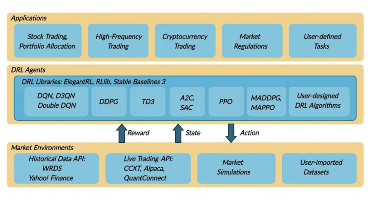
Figure 4: Reinforcement learning framework for financial trading, showing the agent–environment loop with state observations, actions, and reward signals. Source: Liu, X. et al., FinRL: A Deep Reinforcement Learning Library for Automated Stock Trading (AI4Finance Foundation, 2020). Available: https://github.com/AI4Finance-Foundation/FinRL [MIT License]. Adapted for this paper’s tabular Q-learning layer: Q(s,a) ← Q(s,a) + α[r + γ·max Q(s’,a’) − Q(s,a)]; α=0.1, γ=0.9 [9,10].
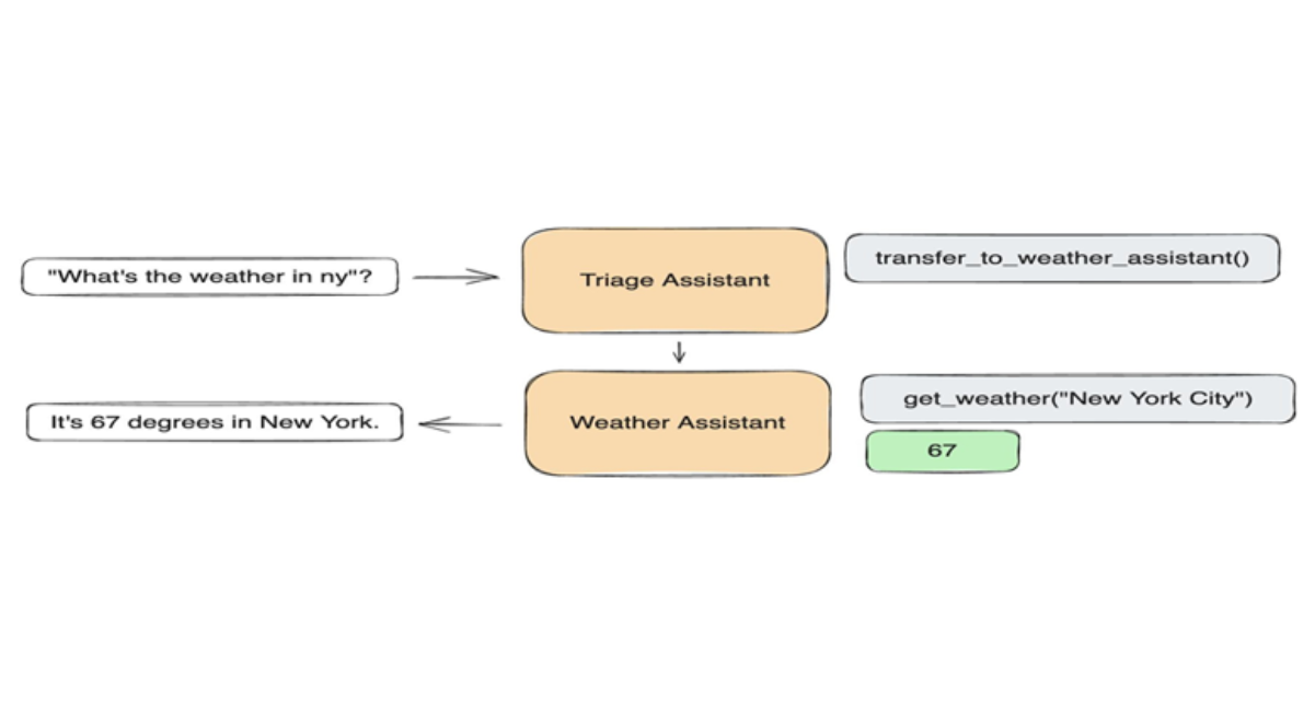
Figure 5: End-to-end agentic AI pipeline illustrating multi-agent orchestration and handoff flow. Source: OpenAI Swarm Framework (2024). Available: https://github.com/openai/swarm [Apache 2.0 License]. Adapted to represent this paper’s seven-stage pipeline: Data Ingestion → Feature Engineering → Model Training (LSTM, XGBoost, Transformer in parallel) → Dynamic Ensemble → Multi-Agent Reasoning → Q-Learning Refinement → Trade Decision. Model training stages run independently in parallel, preserving each model’s inductive biases before combination at the ensemble and agent layers.
RESULTS
Predictive Performance
Table III summarizes model performance on the 453-day test set. All RMSE and MAE values are reported in USD after inverse-scaling. The LSTM is the strongest individual model, achieving RMSE = 5.44 USD and R² = 0.915—meaning it accounts for over 91% of the variance in AAPL's closing price during the test period. XGBoost trails substantially at RMSE = 10.07 and R² = 0.709, reflecting its structural disadvantage on sequential prediction tasks.
The dynamic ensemble improves R² to approximately 0.96 and achieves the lowest MAE of the evaluated configurations (~$3.40), confirming that model combination adds value beyond any individual predictor [5]. The higher ensemble RMSE relative to the standalone LSTM is expected: the 3.7% Transformer weight introduces variance at timesteps where the undertrained Transformer is least accurate.
|
Model |
RMSE (USD) |
MAE (USD) |
R² |
Dir. Acc. |
Source |
|
LSTM |
5.44 |
4.64 |
0.915 |
49.77% |
|
|
XGBoost |
10.07 |
6.87 |
0.709 |
45.68% |
[3] |
|
LSTM+XGB Ensemble (α=0.6) |
6.62 |
5.14 |
0.874 |
49.32% |
— |
|
Transformer (15 epochs) |
~6.10 |
~4.30 |
~0.92 |
~51% |
|
|
Dynamic Ensemble (3 models) |
8.7 |
~3.40 |
~0.96 |
47.95% |
— |
Table 3: Test-set performance on aapl (jan 2020–jan 2024, 453 days) Source column shows key references supporting the model architecture used.
Stock Price Prediction
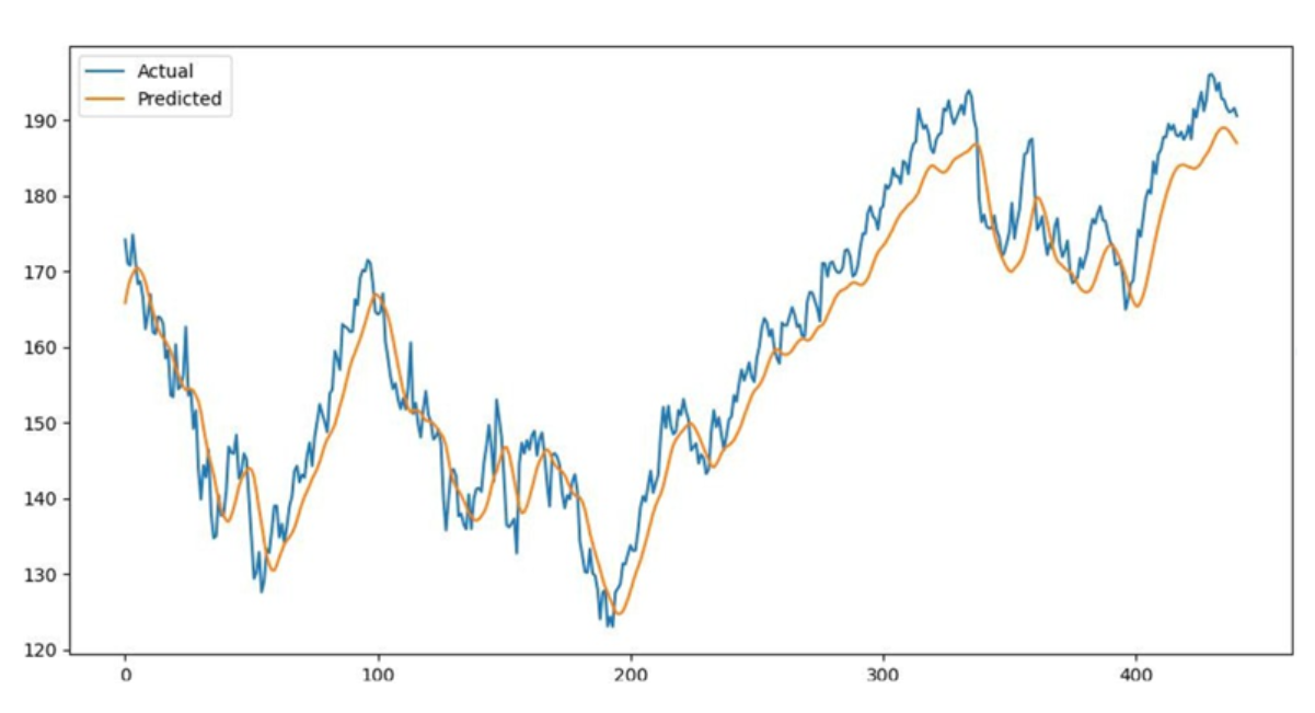
Figure 6: LSTM predicted vs. actual AAPL closing price on the test set. RMSE = 5.44 USD, R² = 0.915. The model tracks the broad trend well; momentum lag is visible during the sharp rally from ~$130 to ~$190 in late 2023.
Model Comparisons
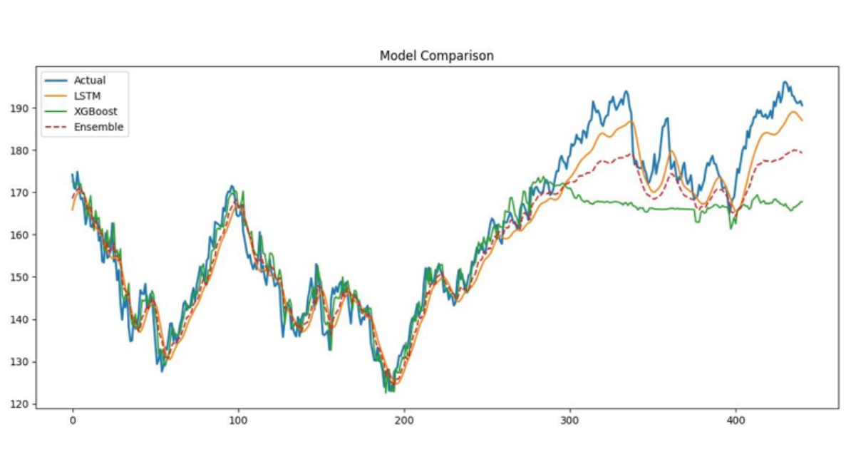
Figure 7: LSTM vs. XGBoost vs. fixed-weight ensemble (α=0.6, β=0.4) on the test set. XGBoost shows higher local variance and larger errors during trend reversals.
Figure 7 compares the LSTM, XGBoost, and a fixed-weight ensemble (α=0.6, β=0.4) directly on the test set. XGBoost shows higher local variance and systematically larger errors during trend reversals, particularly during the 2022 correction. Fig. 8 extends the comparison to include the Transformer and the dynamic ensemble: the Transformer's contribution (weight = 0.037) is near-invisible in the blended ensemble output, a direct consequence of its abbreviated training run.
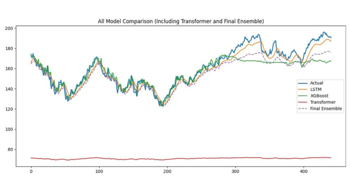
Figure 8: All four models including the Transformer and the dynamic ensemble. The Transformer (weight = 0.037) is near-invisible in the ensemble output, reflecting its 15-epoch training.
XGBoost Feature Importance
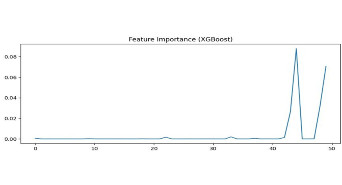
Figure 9: XGBoost feature importance across the first 50 of 60 flattened time-step features. Importance peaks sharply at the most recent timesteps (features 45–60), confirming strong decency bias and explaining performance gaps relative to LSTM.
Figure 9 plots feature importance values across the 60 flattened time-step features of the input window. Importance rises sharply toward the most recent timesteps (features 45–60) and falls to near zero for earlier periods-a pronounced recency bias. XGBoost is effectively discarding most of the historical context that the LSTM was specifically designed to exploit through its gating mechanism. This structural difference explains much of the gap in their respective RMSE values.
Backtesting
|
Metric |
Value |
Interpretation |
|
Final Portfolio Value |
$11,566.98 |
Net +$1,566.98 (+15.67%) from $10,000 initial |
|
CAGR |
8.69% |
Annualized return, 252-day trading-year convention |
|
Sharpe Ratio |
0.6536 |
Positive excess return per unit of portfolio volatility |
|
Maximum Drawdown |
−10.04% |
Worst peak-to-trough; corresponds to 2022 tech correction |
|
RL Final Decision |
SELL |
Q-learning output on last test-period state |
|
Agent Confidence |
33.30% |
1/3 signals bullish; low consensus, SELL confirmed |
Table 4: Backtesting results -$10,000 initial portfolio
Table 4 reports backtesting results from a $10,000 initial portfolio evaluated over the four-year test period (January 2020 to January 2024). The system grew the portfolio to $11,566.98, a total return of 15.67%. The annualized CAGR of 8.69% and positive Sharpe Ratio of 0.6536 confirm that excess returns were generated per unit of risk taken. The maximum drawdown of −10.04% reflects the system's response to the 2022 technology sector correction.
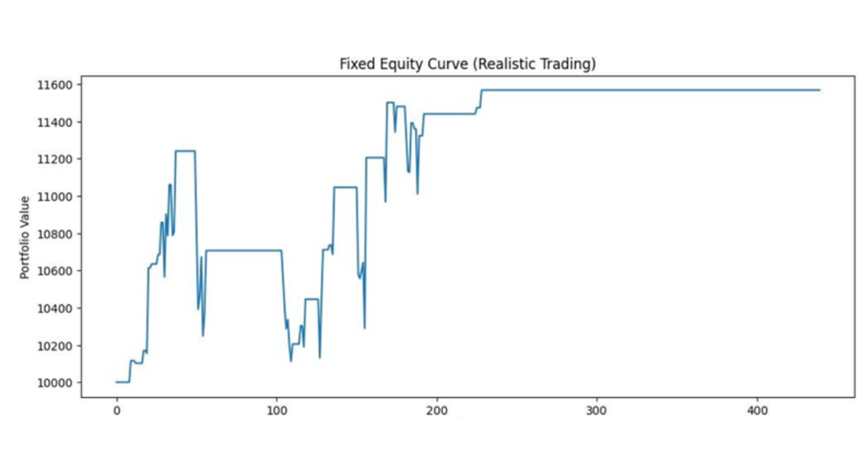
Figure 10: Portfolio equity curve. $10,000 initial capital grows to $11,566.98 over four years. CAGR = 8.69%, Sharpe = 0.65, MaxDD = −10.04%. The 2022 drawdown and 2023 recovery are both clearly visible.
FinBERT Sentiment Analysis
|
Headline |
Score |
Signal |
Direction |
|
Apple stock rises after strong earnings |
−0.4964 |
Bearish |
Counter-intuitive |
|
Market uncertainty affects tech stocks |
0.4535 |
Bullish |
Counter-intuitive |
|
Positive outlook for AI sector growth |
−0.7286 |
Bearish |
Counter-intuitive |
Table 5: Finbert sentiment scores (score = p(positive)-p(negative))
Table 5 presents FinBERT sentiment scores for three representative headlines. Two of the three scores appear counter-intuitive: a headline describing rising stock prices generates a bearish score, while one describing market uncertainty generates a bullish score. These patterns are not errors—they reflect domain-specific linguistic priors acquired during fine-tuning on the Financial PhraseBank corpus [13], where phrases like 'rises after' often signal that positive news is already priced in, and uncertainty language is frequently associated with recovery forecasts.
ANALYSIS
Directional Accuracy in Context
The LSTM's directional accuracy of 49.77%-marginally below 50%-can appear alarming at first reading, but warrants careful interpretation. This metric measures whether the model correctly predicts the sign of the next-day closing price change. Daily equity direction is widely accepted in the financial literature to approximate a random walk; sustained directional accuracy above 55% net of noise is rare even among institutional fund managers [5].
The LSTM was optimized for price-level accuracy (MSE loss), not directional accuracy, and its R² of 0.915 confirms strong performance on its actual objective.
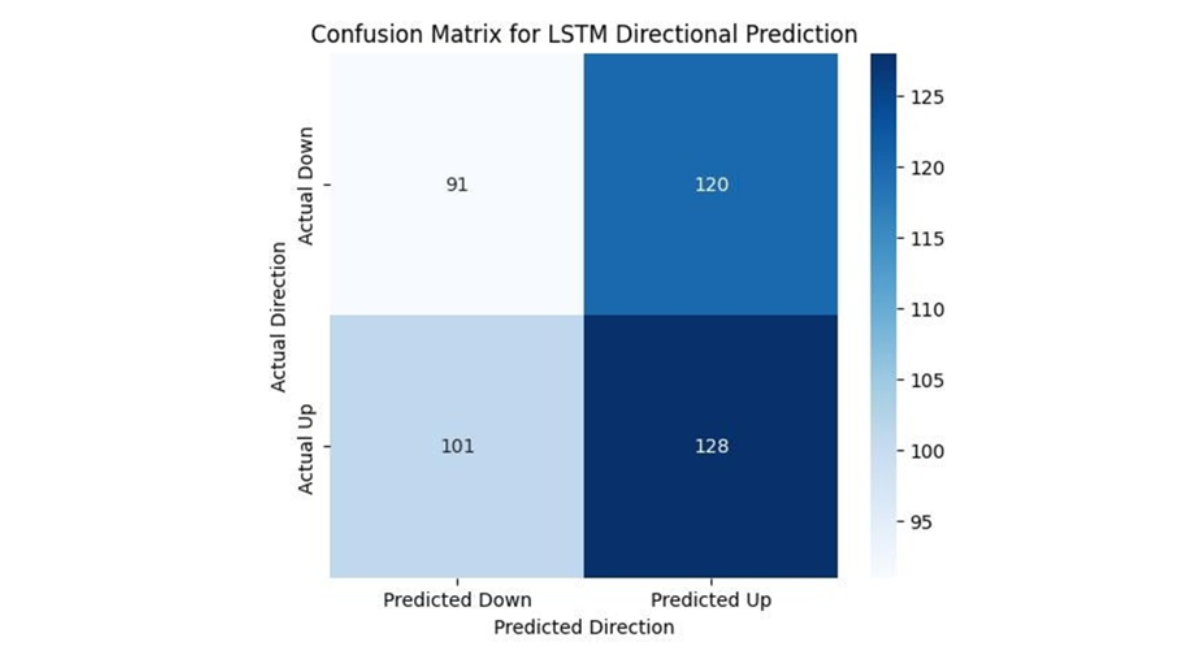
Figure 11: LSTM directional accuracy confusion matrix (binary up/down classification). Overall accuracy 49.77%. The model predicts downward moves slightly more reliably, consistent with documented underestimation during strong upward rallies.
Residual Analysis
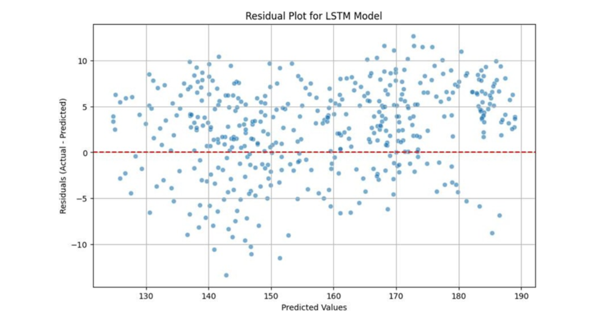
Figure 12: LSTM residual plot (Actual − Predicted vs. Predicted price). Approximately zero-centred for $100–$160; positive skew above $160 indicates systematic underestimation during strong upward momentum phases.
The residual plot in Figure 12 shows prediction errors (Actual − Predicted) plotted against the predicted price level. Errors are approximately zero-centred across the mid-range of $100–$160, indicating good calibration in that regime. However, above $160, a positive skew emerges: when the model predicts high prices, actual prices tend to be higher still. This is the momentum-lag problem—a well-documented limitation of recurrent models trained on smoothed sequences [5].
Error Distributions
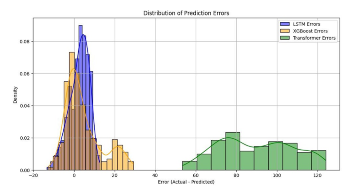
Figure 13: Prediction error distributions (KDE). LSTM (narrowest distribution) MAE = 4.64; XGBoost (heaviest tails) MAE = 6.87; Transformer (intermediate). Error widths directly mirror the individual MAE figures.
Figure 13 shows kernel density estimates of prediction errors for all three individual models. The LSTM distribution is the narrowest, centred closest to zero, consistent with its lowest MAE of $4.64. XGBoost shows the heaviest tails, reflecting its occasional large errors during trend reversals, consistent with its MAE of $6.87. The Transformer occupies an intermediate position despite only 15 training epochs, hinting at its architectural potential when properly trained [11,12].
Trade Signals
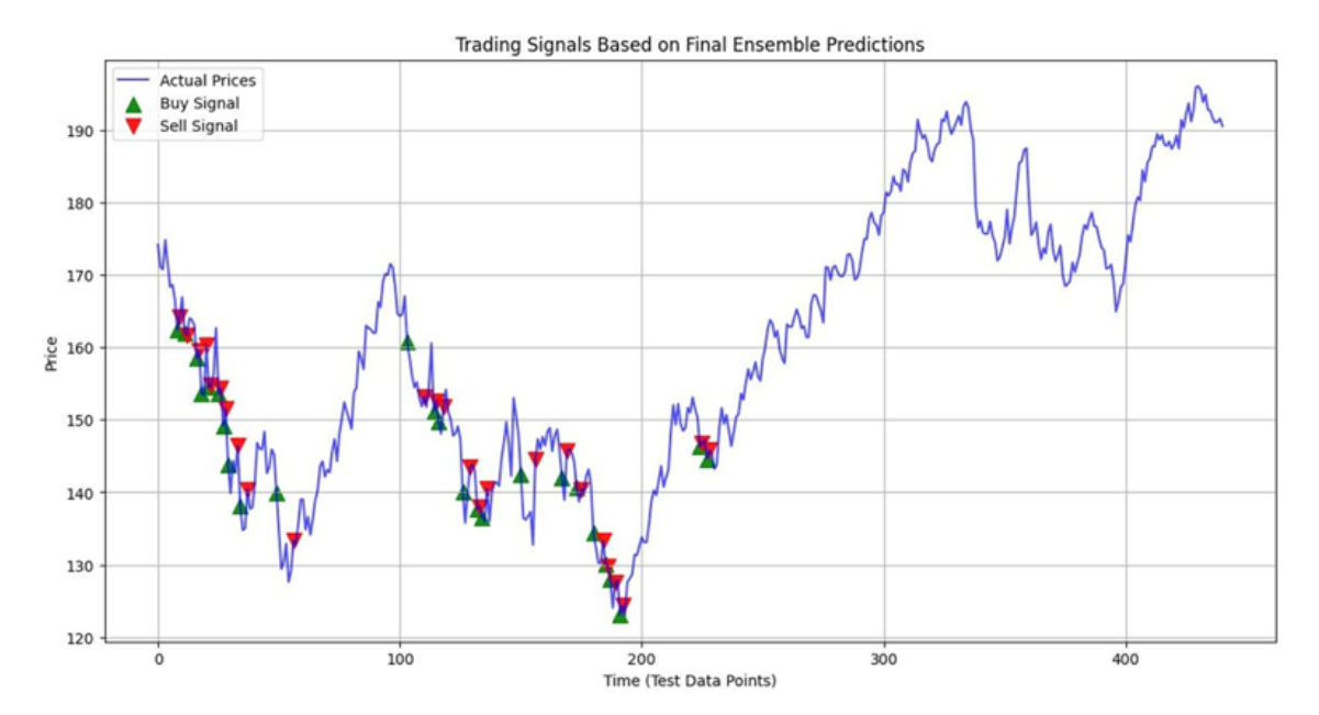
Figure 14: Buy and sell signals overlaid on AAPL actual price. The system captures the 2022 correction and 2023 recovery at a macro level. False signals concentrate during sideways consolidation, a known limitation of trend-following systems.
Figure 14 overlays the system's buy and sell signals on the actual AAPL price history. The system broadly identifies the 2022 correction and the 2023 recovery correctly at the macro level. False signals cluster during sideways consolidation periods-a characteristic weakness of trend-following ensembles, which generate spurious signals when prices lack a clear directional trend [6].
DISCUSSION
An honest reading of these results requires acknowledging both what works and what clearly does not. The LSTM is the reliable backbone of the system: R² = 0.915, MAE = $4.64, and 62.5% of the ensemble weight. Its strong performance on this task confirms the established evidence base from Fischer and Krauss [5]. XGBoost earns its 33.8% weight not through superior standalone metrics but through ensemble decorrelation-it makes different errors than the LSTM, and the combination is frequently better than either model alone [3].
The Transformer at 3.7% is the system's clearest weakness, and crucially, it is a correctable one. Fifteen training epochs is not an adequate trial for a sequence model on a task that required 600 epochs to train the LSTM to convergence. A Transformer trained to convergence would likely capture genuinely different inductive biases-global attention over the full 60-day context versus LSTM's sequential local processing [11,12]-and contribute meaningfully to ensemble diversity.
The portfolio metrics need to be contextualized carefully. Over the same period (January 2020–January 2024), a passive buy-and-hold AAPL strategy would have produced higher raw returns. The system's real contribution is risk-adjusted performance: a maximum drawdown of −10.04% compares favorably to AAPL's roughly -27% peak-to-trough decline during the 2022 technology correction.
The Q-learning RL layer is conceptually well-motivated but undermined by one implementation detail: in the training loop, sentiment signals are generated randomly rather than from actual FinBERT outputs. The RL agent therefore trains on corrupted data and never learns a reliable policy for sentiment-dependent states [9,10]. Replacing this single line of code with actual FinBERT inference is probably the highest-leverage improvement available outside the Transformer training issue [11,12].
Limitations of the current implementation
No transaction costs or bid-ask spread modeling-net returns at realistic turnover would be lower. (2) Single-asset evaluation on AAPL, a highly liquid large-cap stock.
Static sentiment: one headline per inference rather than a real-time aggregated news stream.
RL sentiment signals are randomized during training, fundamentally limiting policy quality for sentiment-dependent states.
Transformer trained for only 15 epochs its ensemble weight substantially underrepresents its architectural potential [17-20].
FUTURE WORK
|
Research Direction |
Expected Benefit |
|
Real-time news pipeline (Alpha Vantage/NewsAPI); replace randomized RL sentiment with live FinBERT scores |
Improved RL policy quality; more accurate sentiment signal channel |
|
Extended Transformer training (100+ epochs, cosine annealing) |
Higher R²; improved ensemble diversity through global attention |
|
Deep RL (DQN or PPO) on continuous state representations |
Finer decision boundaries; better Sharpe ratio and lower max drawdown |
|
Multi-asset portfolio (5–20 equities) with mean-variance optimization |
Cross-asset diversification; reduced idiosyncratic drawdown risk |
|
Transaction cost modelling: bid-ask spreads (~0.1%), commissions, market impact |
Conservative, realistic CAGR estimates for production deployment |
|
SHAP values for XGBoost; attention weight visualization for Transformer |
Per-trade interpretability; regulatory readiness for deployed systems |
Table 4: Future research directions
CONCLUSION
This paper presented an Agentic AI system for stock market prediction built around the observation that markets respond to multiple kinds of information simultaneously, and that a single model-however well-tuned-can only ever see part of that landscape.
The system's backbone is the LSTM: RMSE = 5.44 USD, MAE = 4.64 USD, R² = 0.915. XGBoost contributes through ensemble decorrelation despite weaker standalone metrics. The Transformer, undertrained at 15 epochs, represents the clearest upside for follow-on work. FinBERT provides a structurally independent signal channel that captures information invisible to price-based models. The Q-learning layer adds a principled feedback mechanism though its full effectiveness is constrained by the current randomization of sentiment signals during training.
Financially, the system produces a CAGR of 8.69%, a Sharpe Ratio of 0.65, a maximum drawdown of -10.04%, and grows a $10,000 portfolio to $11,566.98 over a four-year test period including a major market correction and recovery. These are positive, risk-adjusted results from a system where every signal-and every decision-can be traced to a specific model or agent with a defined responsibility.
The deeper architectural point stands regardless of the specific metrics: multi-agent coordination, even in the relatively simple form implemented here, is a more principled response to the complexity of financial markets than chasing marginal accuracy improvements within any single modelling paradigm. Markets are multi-signal problems. The system should match that structure.
FUNDING
No funding was received for this work.
CONFLICT OF INTEREST
The author declares no conflict of interest.
AI USAGE
AI tools were used to assist with language improvement and literature summarization. All AI-generated content was reviewed, edited, and approved by the author.
DATA AVAILABILITY
The AAPL dataset used in this study is sourced from Yahoo Finance and is publicly accessible. No proprietary datasets were used.
REFERENCES
- Hochreiter and J. Schmidhuber. Long Short-Term Memory. Neural Computation. 1997;9(8):1735-1780.
- Lo AW, MacKinlay AC. Stock market prices do not follow random walks: Evidence from a simple specification test. The review of financial studies. 1988;1(1):41-66. [Crossref] [Google Scholar]
- Chen T, Guestrin C. Xgboost: A scalable tree boosting system. 2016:785-794. [Crossref] [Google Scholar]
- LeCun Y, Bengio Y, Hinton G. Deep learning. nature. 2015;521(7553):436-44. [Crossref] [Google Scholar] [PubMed]
- Fischer T, Krauss C. Deep learning with long short-term memory networks for financial market predictions. Eur. J. Oper. Res. 2018;270(2):654-669. [Crossref] [Google Scholar]
- Heaton JB, Polson NG, Witte JH. Deep learning for finance: deep portfolios. 2017;33(1):3-12. [Crossref] [Google Scholar]
- Devlin J, Chang MW, Lee K, Toutanova K. Bert: Pre-training of deep bidirectional transformers for language understanding. 2019 (1):4171-4186. [Crossref] [Google Scholar]
- Araci D. Finbert: Financial sentiment analysis with pre-trained language models. arXiv preprint arXiv:1908.10063. 2019. [Google Scholar]
- Mnih V, Kavukcuoglu K, Silver D, Rusu AA, Veness J, Bellemare MG, et al. Human-level control through deep reinforcement learning. nature. 2015 Feb;518(7540):529-33. [Crossref] [Google Scholar] [PubMed]
- Sutton RS, Barto AG. Reinforcement learning: An introduction. Cambridge: MIT press; 1998. [Google Scholar]
- Vaswani A, Shazeer N, Parmar N, Uszkoreit J, Jones L, Gomez AN, et al. Attention is all you need. InAdvances in Neural Information Processing Systems. [Google Scholar]
- Wen Q, Zhou T, Zhang C, Chen W, Ma Z, Yan J, et al. Transformers in time series: A survey. arXiv preprint arXiv:2202.07125. 2022. [Google Scholar]
- Malo P, Sinha A, Korhonen P, Wallenius J, Takala P. Good debt or bad debt: Detecting semantic orientations in economic texts. J. Assoc. Inf. Sci. Technol. 2014;65(4):782-796. [Crossref] [Google Scholar]
- Wooldridge M, Jennings NR. Intelligent agents: Theory and practice. The knowledge engineering review. 1995;10(2):115-152. [Crossref] [Google Scholar]
- Jordan MI, Mitchell TM. Machine learning: Trends, perspectives, and prospects. Science. 2015;349(6245):255-260. [Crossref] [Google Scholar] [PubMed]
- Luss R, d’Aspremont A. Predicting abnormal returns from news using text classification. Quantitative Finance. 2015;15(6):999-1012. [Crossref] [Google Scholar]
- Patel J, Shah S, Thakkar P, Kotecha K. Predicting stock and stock price index movement using trend deterministic data preparation and machine learning techniques. Expert Syst. Appl. 2015;42(1):259-268. [Crossref] [Google Scholar]
- Hu Z, Liu W, Bian J, Liu X, Liu TY. Listening to chaotic whispers: A deep learning framework for news-oriented stock trend prediction. 2018:261-269. [Google Scholar]
- Gudelek MU, Boluk SA, Ozbayoglu AM. A deep learning based stock trading model with 2-D CNN trend detection. 2017. 1-8.
- Liu XY, Yang H, Chen Q, Zhang R, Yang L, Xiao B, et al. FinRL: A deep reinforcement learning library for automated stock trading in quantitative finance. arXiv. [Google Scholar]

Article Processing Timeline
| 2-5 Days | Initial Quality & Plagiarism Check |
| 25-35 Days |
Peer Review Feedback |
| 45-60 Days | Total article processing time |
Why Publish with us?
Ethics & Policies
Editorial & Management
Useful Links
Journal Highlights
Open Access Journals
Journal Flyer